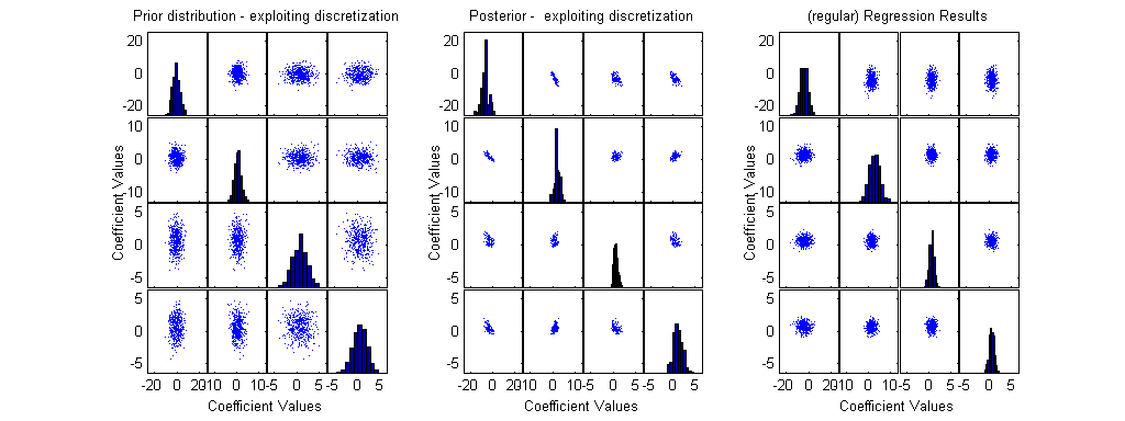
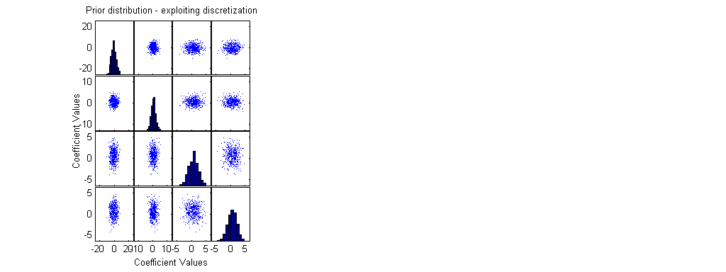
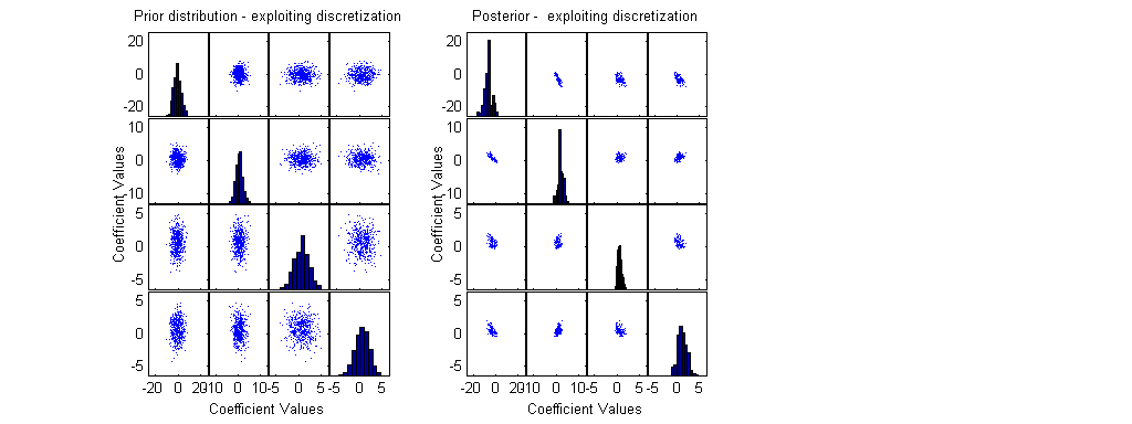
Bayesian Analysis for a Poisson response GLM

We suggst a method which allows estimation of posterior information even when the closed form of the posterior is very complex, exploiting a discretization of the prior distribution.

This need for posterior distribution is quite frequent, and we use it for the purpose of analyzing small sample data with generalized linear models. Using regression techniques for GLM with small samples is not reliable, and often highly biased.

The sequential experimental design examples already contain this utilization; here this idea is given a seperate example, for ready-made data.

This file contains a Poisson example. X0 contains the location of the experiment, RResult contains the responses observed.

We provide 3 plots: (1) A presentation of the prior, by a sample of possible discrete points; (2) A presentation of the posterior, by discrete points; (3) A sample of possible coefficient values, from analysis through regression (GLM).

This script was written by Hovav Dror, Tel-Aviv University, 2006

If you make changes to the script, or if you implement it to a (to be) published problem, please inform us: dms@post.tau.ac.il ; hovavdror@gmail.com

further details, including papers describing the algorithm, can be found at: http://www.math.tau.ac.il/~dms/GLM_Design

Prior Distribution
Data:
Plot of the prior distribution
Calculate the Weights
Posterior
Regular Regression (GLM)

Prior Distribution

NN=10000; % Number of parameter vectors to represent the prior using a discretization
m=3; p=4;
BetaMeans=[   -0.7   0.5   0.7   0.7];
BetaSE=[3 1.5 1.5 1.5];
NI=rand(NN,p);
beta = norminv(NI,ones(NN,1)*BetaMeans,ones(NN,1)*BetaSE);

family='poisson';
link='log';
model='linear';

Data:

Locations

X0=[
    0 0 2
    2 2 0
    2 0 2
    2 2 2
    1 3 3
       ];
F0=x2fx(X0,model);
% Results:
 RResult=[
      0
    1
    1
    3
    3
        ];

Plot of the prior distribution

scrsz = get(0,'ScreenSize');
set(gcf,'Position',[0 scrsz(4) scrsz(3) scrsz(4)/2]); % small figure upper right of the screen
subplot(1,3,1);
[H,AX,BigAx,P] =plotmatrix(beta(1:500,:)); % A sample of 500 points from the prior
xlabel('Coefficient Values');
ylabel('Coefficient Values');
title('Prior distribution - exploiting discretization');
x1=get(AX,'XLim');
y1=get(AX,'YLim');

Calculate the Weights

ResultFactorial=[];
for i=1:length(RResult)
    if RResult(i)<21
        ResultFactorial(end+1)=factorial(RResult(i));
    else
        ResultFactorial(end+1)=-1; % else - use normal approximation and not the exact poisson distribution
    end;
end;

RealMinSS=realmin^(1/length(RResult));
RResultM=ones(NN,1)*RResult';
bx=(F0*beta')';
lambda=exp(bx);
LRi=[];
for i=1:NN
    LRi(i)=0;
    for j=1:length(RResult)
        if lambda(i,j)>20 | RResult(j)>20  % if it is better to use normal approximation
            LRi(i)=LRi(i)  -0.5*log(2*pi*lambda(i,j)) - (RResult(j) - lambda(i,j))^2 / (2*lambda(i,j)) ;
        else % for small lambda & RResult use exact poisson distribution
            LRi(i)=LRi(i) +log( max([lambda(i,j)^RResult(j) * exp(-lambda(i,j)) / ResultFactorial(j) RealMinSS]));
        end; % if lambda
    end; % for j
end; % for i

MaxLogLike=max(LRi);
MinLogLike=min(LRi);
LRealMin=log(realmin);
if MinLogLike<LRealMin
    ScaleAddition=LRealMin-(MinLogLike-MaxLogLike);
    LRi=LRi+ScaleAddition;
    MaxLogLike=max(LRi);
end;

if exp(MaxLogLike)>0 % if max likelihood is computable
    LRi1=exp(LRi-MaxLogLike);
    LRi1=LRi1/sum(LRi1);
else
    fprintf('\nMax Likelihood =0 ! \n');
end;

Weights=LRi1';

Posterior

Wbeta=sortrows([Weights beta]);
SW=cumsum(Wbeta(:,1));
beta1=Wbeta(SW>0.05,2:end); % Posterior possible beta values, for a 95% level
Weights1=Wbeta(SW>0.05,1);

Sample1=randsample(length(Weights1),500,true,Weights1); % Choose a Weighted sample of size 500
subplot(1,3,2);
[H2,AX2,BigAx2,P2] =plotmatrix(beta1(Sample1,:));
for i=1:p
    for j=1:p
    set(AX2(j,i),'XLim',x1{(i-1)*p+1});
    set(AX2(i,j),'YLim',y1{i});
    end;
end;
title('Posterior -  exploiting discretization');
xlabel('Coefficient Values');
ylabel('Coefficient Values');

Regular Regression (GLM)

subplot(1,3,3);
  [b,dev,stats] = glmfit(X0,RResult,'poisson');
  NI2=rand(500,p);
beta2 = norminv(NI2,ones(500,1)*b',ones(500,1)*stats.se');
[H3,AX3,BigAx3,P3] =plotmatrix(beta2);
for i=1:p
    for j=1:p
    set(AX3(j,i),'XLim',x1{(i-1)*p+1});
    set(AX3(i,j),'YLim',y1{i});
    end;
end;
title('(regular) Regression Results');
xlabel('Coefficient Values');
ylabel('Coefficient Values');