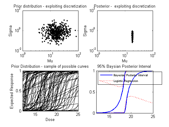
Bayesian Posterior Interval allows interpretation of data. We suggst a method which allows estimation of posterior information even when the closed form of the posterior is very complex, exploiting a discretization of the prior distribution.
This need for posterior distribution is quite frequent, and we use it for the purpose of analyzing small sample data with generalized linear models. Using regression techniques for GLM with small samples is not reliable, and often highly biased.
The sequential experimental design examples already contain this utilization; here this idea is given a seperate example, for ready-made data.
This file contains a binomial example. X0 contains the location of the experiment, RResult contains the responses observed (0/1).
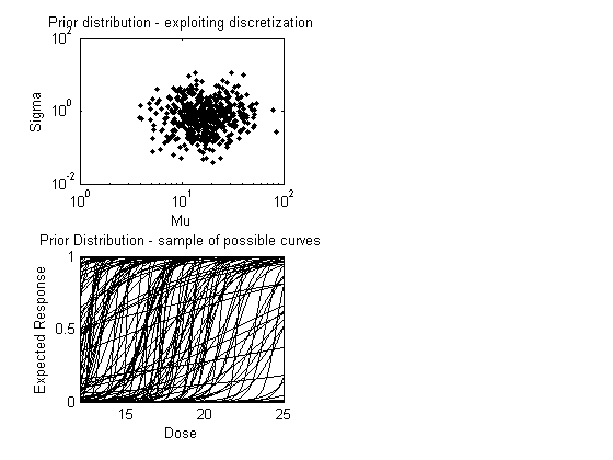
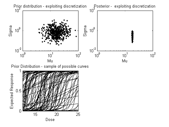
We provide 4 plots: (1) A presentation of the prior, by a sample of possible discrete points; (2) A presentation of the posterior, by discrete points; (3) A presentation of the prior by a sample of possible curves; (4) A presentation of the posterior interval vs. logistic regression confidence interval.
This script was written by Hovav Dror, Tel-Aviv University, 2006
If you make changes to the script, or if you implement it to a (to be) published problem, please inform us: dms@post.tau.ac.il ; hovavdror@gmail.com
further details, including papers describing the algorithm, can be found at: http://www.math.tau.ac.il/~dms/GLM_Design
NN=10000; % Number of parameter vectors to represent the prior using a discretization
% If not much is known, you can use a very rough prior, for example:
MedianMean=17;
MuS=lognrnd(log(MedianMean),0.5,NN,1);
MedianSigma=0.7;
SigmaS=lognrnd(log(MedianSigma),1,NN,1);
beta=[-MuS./SigmaS  1./SigmaS];
family='binomial';
link='logit';
model='linear';
Locations
X0=[  17.0000
   22.5000
   19.4000
   19.1000
   16.4000
   17.9000
   18.4500
   17.2000
   18.8000
   19.8000
   18.5500
   19.7500
   18.7000
   17.6200
   19.4000
   17.8400
   18.0000
   19.1500
   18.1100
   ];
F0=x2fx(X0);
% Results:
RResult=[   0
     1
     1
     1
     0
     0
     1
     0
     0
     1
     0
     1
     1
     0
     1
     0
     0
     1
     0
     ];
subplot(2,2,1);
loglog(MuS(1:500),SigmaS(1:500),'k.');% A sample of 500 points from the prior, log-scale
xlabel('Mu'); ylabel('Sigma');
title('Prior distribution - exploiting discretization');
x1=get(gca,'XLim');
y1=get(gca,'YLim');

subplot(2,2,3);
xrange0=[12 25];
plot([xrange0(1) xrange0(1) xrange0(2)],[0 0 1],'w'); % empty figure
hold on
P=[];
for ii=1:150 % Plot a sampe of 150 possible curves, from the prior
    j=0;
    xrange=min([min(X0) xrange0(1)]):.01:max([max(X0) xrange0(2)]); % range for plotting figures
    for x=xrange
        j=j+1;
        P(j)=1 / (1 + exp(-beta(ii,1)-beta(ii,2)*x) );
    end;
    plot(xrange,P,'k');
end; %for
hold off
set(gca,'XLim',xrange0);
xlabel('Dose');
ylabel('Expected Response');
title('Prior Distribution - sample of possible curves');
RResultM=ones(NN,1)*RResult';
ex=exp(-F0*beta');
bprob=(1 ./ (1+ex))';
mprob=1-bprob;
LRi = prod( bprob.^RResultM ,2 ) .* prod( mprob.^(1-RResultM) ,2);
Weights=LRi/sum(LRi);
WMuSig=sortrows([Weights MuS SigmaS]);
SW=cumsum(WMuSig(:,1));
MuSig1=WMuSig(SW>0.05,2:end); % Posterior possible beta values, for a 95% level
Weights1=WMuSig(SW>0.05,1);

Sample1=randsample(length(Weights1),500,true,Weights1); % Choose a Weighted sample of size 500
subplot(2,2,2);
loglog(MuSig1(Sample1,1),MuSig1(Sample1,2),'k.');% A sample of 500 points from the posterior, log-scale
xlabel('Mu');
ylabel('Sigma');
set(gca,'XLim',x1);
set(gca,'YLim',y1);
title('Posterior -  exploiting discretization');
xrange=min([min(X0) xrange0(1)]):.1:max([max(X0) xrange0(2)]); % range for plotting figures
Wbeta=sortrows([Weights beta]);
SW=cumsum(Wbeta(:,1));
beta1=Wbeta(SW>0.05,2:end);
P=[];
LL=ones(size(xrange));
UL=zeros(size(xrange));
i=0;
for x=xrange
    i=i+1;
    for j=1:length(beta1)
        P=1 / (1 + exp(-beta1(j,1)-beta1(j,2)*x) );
        if P<LL(i), LL(i)=P; end;
        if P>UL(i), UL(i)=P; end;
    end;
end;

subplot(2,2,4);
h1=plot(xrange,LL,'LineWidth',2);
hold on
plot(xrange,UL,'LineWidth',2);
hold off;
title('95% Baysian Posterior Interval');

% And add a comparison to logistic regression (dotted red lines);
[b,dev,stats] = glmfit(X0,[RResult ones(size(RResult))],'binomial');
[yfit,dlo,dhi] = glmval(b,xrange','logit',stats,0.95);
hold on
h2=plot(xrange,yfit-dlo,'r:','LineWidth',2);
plot(xrange,yfit+dhi,'r:','LineWidth',2);
hold off
set(gca,'XLim',xrange0);
h_legend=legend([h1 h2],'Bayesian Posterior Interval','Logistic Regression');
h_text = findobj(h_legend,'type','text');
set(h_text,'FontUnits','points','FontSize',7)
set(h_text,'FontUnits','normal')
set(h_legend,'Location','NorthWest');
set(h_legend, 'Color', 'none')