Reinforcement Learning – Final
Project: A Learning Traffic
Light
Submitted by Libi Hertzberg and Yossi Mossel as part of the requirements for the course Reinforcemnet Learning given by Professor Yishay Mansour in fall 1999.
Introduction:
In our project we aim to create an algorithm for learning an efficient policy for managing traffic in a four way junction. The project consists of a junction simulator and a learning algorithm implementing SARSA learning. It was implemented in Visual C++ 6.0.
The
Junction Simulation:
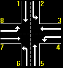
The junction model is a four way junction in which from each direction it is possible to drive either straight or turn left (a right turn can be made whenever going straight). Each way is divided into two lanes – one for each possible direction. The rate of incoming traffic into a lane is a poissonically[1] distributed random variable, whilst the rate of out going traffic is a constant. Both these parameters are determined by the user for each lane independently. The junction has eight possible configurations of the traffic lights, these are:
Configuration 1: Lanes 1 & 2.
Configuration 2: Lanes 1 & 5.
Configuration 3: Lanes 2 & 6.
Configuration 4: Lanes 3 & 7.
Configuration 5: Lanes 3 & 4.
Configuration 6: Lanes 4 & 8.
Configuration 7: Lanes 5 & 6.
Configuration 8: Lanes 7 & 8.
The simulation updates the state of the junction every five seconds (simulation time). In an update incoming traffic is added to the current number of cars in each lane according to the given rate. For the two lanes which are active in the current configuration, the number of outgoing cars is subtracted. To determine what should be the next configuration the simulation queries the policy computed so far by the algorithm. Each configuration change carries with it a “fine” of three dead seconds in lanes which change from unactive to active.
The
Learning Algorithm:
In reinforcement learning the learning agent acts in an environment which is influenced by its actions. The learning process uses a Markovian Decision Process (MDP).
The MDP consists of the following:
- A set S of states which mirror the current “location” in the environment.
- A set A of actions possible. These actions are a mapping of the actions possible in the environment.
- A transition function d: S´A´S à [0, 1], giving the probability of reaching a state S ' s’ from state S ' s having taken action A ' a.
- A reward function R: S´Aà Â. Giving for each state and action an immediate reward.
- A policy function Õ: S à A. Choosing for each state the action to be done.
In our model the MDP is:
- States:
When defining our states we use only information which it seems reasonable to assume that an actual system
could have access to. In our model the learning agent has six detectors in each way. An activation of a detector means that the way is filled with cars up to the detector’s location. The amount of cars up to the sixth detector is set to 150. Hence, if no detector is activated there are 0 – 25 (150/6) cars in the way. If six are activated there are above 150 cars. We do not detect the traffic per lane as it does not seem technically feasible to do so. A state includes the number of detectors activated in each way, and the current junction configuration.
- Actions:
An action is choosing the next junction configuration.
- Transition function:
Is implicit in our model. Every five seconds the simulation computes its current state. The MDP updates its current state according to the received values.
- Reward:
The reward function aims to achieve a balance between minimizing the number of cars in the junction and prevention of “starvation” i.e. a situation in which the waiting time of a particular lane is extremely large. Its general form is: -S( Xiz * Yiw ). Where Xi is the number of cars in lane i, and Yi is the time since the last green in lane i. The user can determine the weight given to each component by choosing the parameters z and w.
- Policy:
The policy is computed using the SARSA algorithm. SARSA is an on policy algorithm, meaning that it can update the policy used for the learning process. SARSA is used in cases in which the model is such that the transition function d is unknown or hard to compute, but we are able to sample the environment or a model of it. In our case such a sampling is the current state of traffic in the junction computed by the simulation. The algorithm evaluates the value of those pairs of the form (S´A) which are reached during the simulation. This value converges to the optimal value of taking action a in state s. The value represents a weighted average vbetween the immediate reward and the expectation of future states’ values. This future value is discounted using a parameter 0<l<1. The purpose of the discounting is to bound the value in cases of infinite horizon. Furthermore, by the value we assign to l we determine the relative importance given to future states’ values in comparison to the immediate reward. l determines how “far” we look ahead when computing a (state, action) value.
The formula used:
Q(s,a) = Q(s,a) + a[(r(s,a) + lQ(s’, a’) – Q(s,a)]
A learning algorithm should resolve the exploration vs. exploitation dilemma. The problem is how to gain maximum reward (exploitation) while still sampling new actions (exploration). Values computed by the algorithm are still highly random during the beginning of the learning process. Not exploring the states’ field at this stage might result in never reaching states/actions which are highly rewarding. In a later stage of the learning process we would like our algorithm to begin reaping the results. SARSA resolves this dilemma by introducing an element of randomness into the policy. When picking an action, we pick the action with the highest value of all actions possible from the current state. In probability e we pick a random action. This is called an e-greedy policy. As we want our policy to be more explorative during initial phases learning and less so as the run progresses, we use a converging series of epsilons. The value of e is in inverse proportion to the logarithm of the number of seconds since the beginning of the run. In order to not lose completely all exploration by the algorithm we define a lower bound of 0.05 for e.
In a junction of the type that we model there are eight possible configurations (see above). Most conventional traffic lights utilize only four of these (enough to cover all lanes) , in a predetermined cycle. The time alloted for each way is constant, perhaps varying according to the time of day. Our policy is unrestricted. It can change to all possible configurations in any order. We decided upon this implementation as it seems that this rigidity of conventional traffic lights is a major drawback. We bear in mind, that in an actual system this could be problematic, since people are used to be able to predict when their light will turn to green. The only restriction placed is bounding the maximal time between greens in a lane . This is done as we want to be able to guarantee that this bound indeed exists. The reward function should give the same end result, as it considers the waiting time in each lane. Yet, we enforce this as a restriction on the policy as we know in advance that the waiting time in a lane should be bounded. There is no benefit in letting the algorithm achieve the same result.
Results:
1) A simple case – In this case we show the performance of the algorithm on the a junction in which only lane 1 has a high traffic rate. In the learning curve we only show this lane as the amount of traffic on other lanes never reaches a high level. The amount of time given to each configuration after the learning process is shown in the pie chart. Observe that lane 1 is active for 52% of the time (configurations 1 and 2), while the amount of traffic through this lane is 58% of the total amount of traffic in the junction.
![]()
2) A more difficult case: Relatively high amount of traffic in all lanes, two lanes with extremely problematic amount of
traffic.
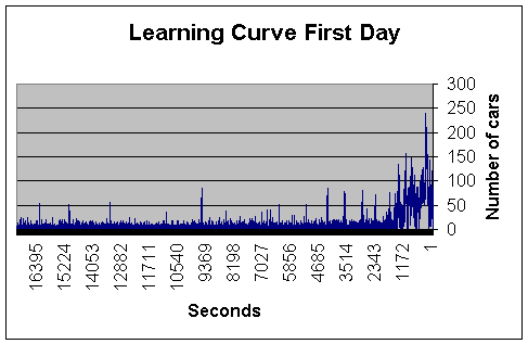
- On the first day of learning the rate of incoming traffic is so high that the amount of traffic in the junction exceeds the MDP’s ability to differentiate between different states. Any number of cars above 150 registers as maximal traffic. As a result, the learning algorithm is “overloaded” and has difficulty in learning in the later parts of the day. In these cases the algorithm requires a high number of learning days to achieve a satisfactory policy.
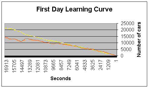
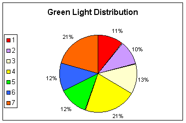
After 250 days of learning we observe the following traffic. The algorithm has managed to learn a policy which stabalizes the junction. The lanes colored orange and yellow are the same as in the figure above.
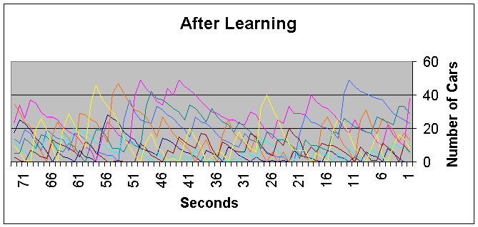
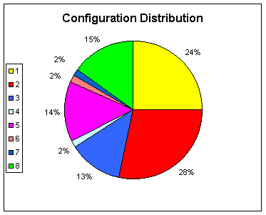
Observe that the problematic lanes are active for twice as much as the other lanes. This agrees with traffic rate on the lanes.
Comparative Results:
The learning algorithm compares extremely favourably when compared to a naïve policy giving equal amounts of time on each lane. To gain more insight on the quality of the SARSA algorithm we compare to what we call the semi–optimal policy. The semi-optimal is similar to conventional traffic lights. It uses four configurations in a predetermined cycle. The time allocated to each way is proportional to its relative part in the total junction traffic. We call this semi-optimal, as if it were used on a deterministic junction (a junction in which the traffic is constant) it would be close to the optimal[2]. It would not be the actual optimal policy as it does not consider each lane separately, but computes the time allocation for each way. We still consider it to be a good indication to what can be achieved for a specific situation.
Our algorithm achieves superior results. This can be due to the following factors:
- Reaction to changing circumstances. Our algorithm should be able to deal effectively with anomalous situations arising in the junction. This is due to the fact that it is not bound to a predetermined cycle of configurations, enabling it to make configuration changes according to the situation at hand.
- There are configuration changes which are better than others. As there is a “dead” time when a lane changes from unactive to active, it is more profitable to use configuration changes in which one lane stays active. Our algorithm could use these “good” changes to minimize the length of dead periods in the junction.
-
|
|
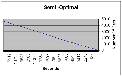
In most cases the semi-optimal achieves reasonable results. However, let us first consider a case in which the semi-optimal algoritm fails, while the RL algorithm succeeds in stabalizing the junction. This is due to the low arrival rate on one of the lanes. It is so low that the semi-optimal policy only assigns it one time segment per cycle. In this case the proportion of “dead” time on the lane is so high (60%), that the amount of traffic on the lane goes out of control.
|
|
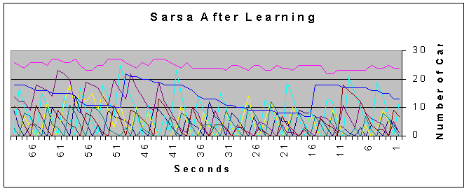
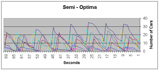
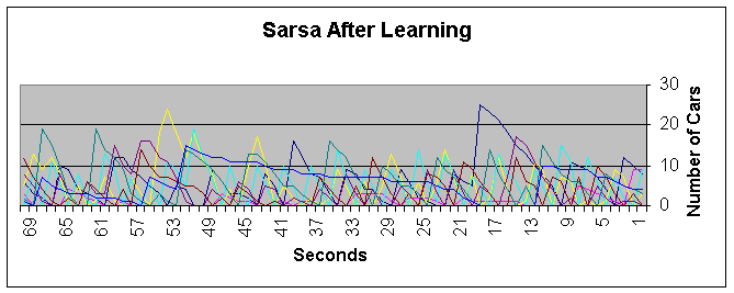
In a more typical case the semi-optimal policy does not perform so poorly. In the following test case, moderate traffic rates are used. The semi-optimal policy does manage to stabalize the traffic through the junction. The traffic on the busiest lane, lane 3 – colored blue, does not exceed 35, and its average value over a period of one day is 7.03 cars. The SARSA algorithm manages to learn a policy in which traffic on lane 3 never exceeds 25 and maintaining an average of 4.54 cars.
|
|
|
|
Conclusion:
- RL techniques can achieve satisfactory results on the traffic light problem. It is difficult to give a full assessment of the quality of our results as we compare our results to a static policy (one not influenced by the current state of affairs in the junction). A more complete analysis would require comparison with a greedy dynamic policy.
- The assessmment of the results is presented with further difficulties as it is not completely clear what an optimal policy must achieve. See footnote [2].
- Parameter tweaking was difficult. This was due to two different factors:
1) The large number of parameters (junction parameters and SARSA parameters) made a systematic search of the
parameter space difficult to achieve manually.
2) Unstable behaviour of the learning algorithm. Very slight changes in the parameters could result in the algorithm
being unable to give a satisfactory solution. For instance, we discovered that for a given junction configuration,
slight changes in the “dead” time in the junction can cause radical changes in the algorithm’s performance. This
might be due to the fact that in situations in which the junction is full, the algorithm is unable to take actions which
change the MDP’s state, as the MDP does not differentiate between different levels of traffic above 150.
If the junction fills up too rapidly there is no learning time on interesting states. Apparently this borderline can be
crossed by very slight changes in the parameters.
- Some of our prior expectations were not realized by the resulting policies. We expected that the algorithm would learn that it is profitable not to change configurations too often, as there is a price to be paid for a configuration change – “dead” junction time. In some situations we did witness this kind of behaviour, but due to the above mentioned problems we were unable to reach conclusive results on the matter.