Andrew Moore
Mary Soon Lee
Brigham Anderson
School of Computer Science
and Robotics Institute
Carnegie Mellon University,
Pittsburgh PA 15213
Summarized by:
School of Mathematical
Science
Tel-Aviv University,
Tel Aviv 69978
ISRAEL
Abstract
The two papers introduce a new algorithm and data structure for quick counting and machine learning datasets. The task of counting is fundamental in the field of machine learning algorithms operating on datasets of symbolic attributes. Therefore, it is important to achieve computational efficiency in it, especially when applied to large datasets. The authors give a very sparse data structure, the ADtree, that minimizes memory use, thus making it applicable to large datasets, and an algorithm operating on it, that is used to construct the contingency table. Under several assumptions, the cost of these operations is shown to be independent of the number of records in the dataset and log-linear in the number of non-zero entries in the contingency table.
The author give an example of applying their method to the
problem of discovering association rules in large datasets. They show how
the method can significantly accelerate exhaustive search of rules compare
to traditional counting, presenting results in a variety of datasets involving
many records and attributes.
1. Caching Sufficient Statistics
Many machine learning algorithms operating on datasets of symbolic attributes need to do frequent counting. The work is also applicable to Online Analytical Processing (OLAP) and Data Mining (DM), where operations on large datasets such as multidimensional databases accesses, DataCube operations and discovering association rules could benefit from fast counting.
Notation:
A query is a set of (attribute = value) pairs in which the left hand sides of the pairs form a subset of {a1, ..., aM}, arranged in increasing order. The total number of queries is (n1 + 1)(n2 + 1) ··· (nM + 1), because each attribute can either appear with one of its values, or it can not appear (having the value ai = * "don't care" value). Some examples of queries are
(a1 = 1); (a2 = 3, a3 = 1); ()
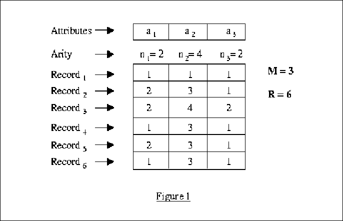
A count of a query, denoted by C(Query) is simply the number of records in the datasets matching all the (attribute = value) pairs in Query. For the above three queries and the dataset given in Figure 1, the count is
C(a1 = 1) = 3
C(a2 = 3, a3 = 1) = 4
C() = 6
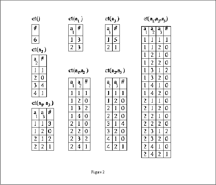
Contingency tables:
Each subset of attributes ai(1) ... ai(n)
has an associated contingency table denoted by ct(ai(1)
... ai(n)). This is a table with a row for each of the possible
sets of values for ai(1) ... ai(n). The row corresponding
to ai(1) = v1, ..., ai(n) = vn
records the count C(ai(1) = v1, ..., ai(n)
= vn)). The dataset in figure 1 has 8 contingency tables (figure
2).
It is quite easy to see that there exists a mechanism that counts in constant time. Simply cache the contingency table for each query. But one must realize that doing so for even very small dataset, could require vast amount of memory. For example, a dataset with 20 attributes each of arity 2, will take (2 + 1)20 ~ 1.5GB of memory.
The ADtree data structure:
Figure 3 describes An ADtree. An ADnode (shown as a rectangle) has child nodes called Vary nodes (shown as ovals). Each ADnode represents a query and stores the number of records that match the query. The Vary aj child of an ADnode has one child for each of the nj values of attribute aj. The kth such child represents the same query as Vary ajs parent, with the additional constraint aj = k.
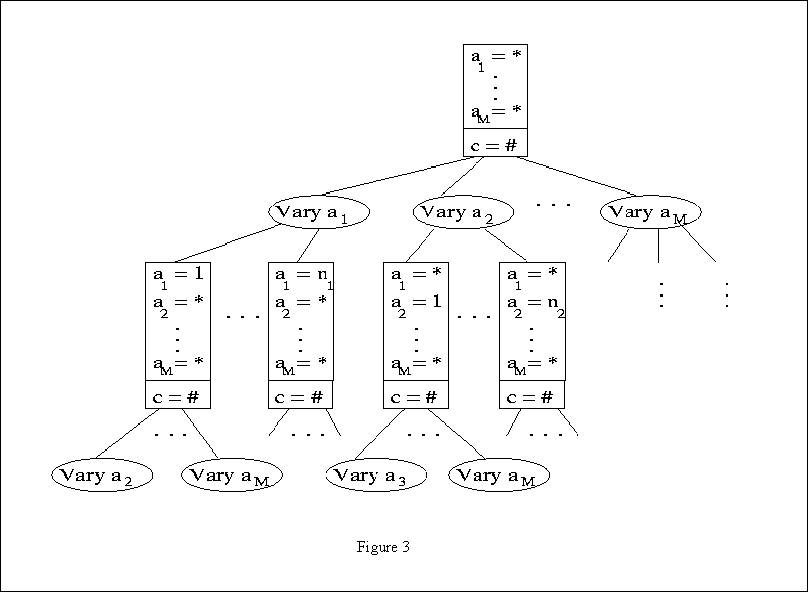
Note that:
because information for Vary nodes with indices below i+1 can be obtained
from an already exist path in the ADtree.
Cache reduction I: cutting off nodes with count zero
We can store a NULL pointer instead of a node for any query
that matches zero records. All of the specializations of such query will
have count zero too. Still, we have (n1 + 1)(n2 +
1) ··· (nM + 1) possible nodes in the worst
case, although in practice it could reduce a considerable amount of memory.
Cache reduction II: the sparse ADtree
Each Vary aj node in the above ADtree stores nj subtrees. Instead, we will find the most common of the values of aj (call it MCV) and store a NULL in place of the MCVth subtree. The remaining nj 1 subtrees do not change. The number of nodes need to be stored in the sparse ADtree, for binary relations, is now bounded by 2M (instead of 3M(, because we omit one value for aj, having at most n1 · n2 ··· nM possible queries. We next show how it is possible to compute a full contingency table from the sparse ADtree.
Computing contingency tables from the sparse ADtree
We are given an ADtree and an arbitrary set of attributes {a1, ... , an} for which we wish to quickly compute the contingency table. Notice that the conditional contingency table ct(ai(1) ... ai(n) | Query) can be built recursively. We first build
ct(ai(2) ... ai(n) | ai(1) = 1, Query)
ct(ai(2) ... ai(n) | ai(1) = 2, Query)
.
.
.
ct(ai(2) ... ai(n) | ai(1) = ni(1),
Query)
and then combine them to one table.
Note to that we do not have to specify the explicit query, but provide the corresponding ADnode of the ADtree.
We can use the above algorithm to obtain ct(ai(2) ... ai(n) | Query) by calling
MakeContab( {ai(2) ... ai(n)}, ADN )
and thus
CTMCV = MakeContab( {ai(2) ... ai(n)}, ADN ) - åk¹ MCV CTk
The complexity of building a contingency table with the above method is given in the following recurrence relation
If we didnt cache any data, we would need O(nR + kn) operations where R is the number of records in the dataset. When we have kn << R we are significantly cheaper then simple full table scans. Since we are interested in large datasets, this result is very promising. The authors show that in datasets where R > 100,000, the improvement achieved is in orders of magnitude.
Leaf-Lists
It is not worth building the ADtree data structure
for a small number of records. Instead, we set a number, Rmin
to be the number of rows under which we do not expand the subtree, but
simply store a set of pointers to the dataset. The major consequence of
this change is that mow the dataset needs to be retained in main memory.
2. Fast Learning of Associations Rules
The problem of discoveringassociation rules in largedatabases hreceived considerable resattention. Complex association rules are capable of representing concepts such as "PurchasedChips = TRUE" and "PurchasedSoda = FALSE" and "CostumerType = OCCASIONAL" => "AgeRange = YOUNG". Such concepts are very useful in data mining applications, for example, and are very intuitive and actionable to work with.
Problem Definition
Define dataset as in the previous section. We define literal as an attribute-value pair such as "education = master". Let L be the set of all possible literals for a dataset. An association rule is an implication of the from S1 => S2 where S1, S1 Î L, and S1, S2 are disjoint.
Each rule has a measure of statistical significance called support. For a set of literal S Î L , the support of S is the number of records in the dataset that match all the attribute-value pairs in S, and is denoted supp(S). We define the support of the rule S1 => S2 to be supp(S1 Ç S2). A measure of the strength of the rule is called confidence, and is defined to be
When the problem is mining association rules to predict user-supplied target set of literals S2, it requires calculating large numbers of rule confidences and supports. We are in for a task of counting through the dataset over and over, for each given predicate of literals. Small improvement in this task will have a great influence on the overall performance.
Figure 4 shows some examples
of different dataset used by the authors to test their improved counting.
The experiments involved using the CN2 algorithm that searches for association
rules, comparing two methods of counting: simple table scan and the ADtree
data structure and algorithm mentioned above. Notice the short building
time of the ADtree and the low amount of memory it consumes.
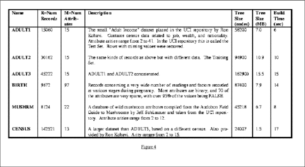
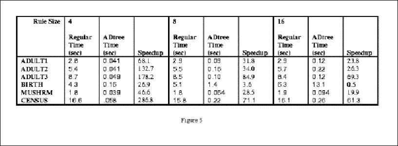
Figure 5 shows some results.
Note also that on all datasets, except for the BIRTH dataset, a significant speedup was achieved. The problem with the BIRTH dataset was due to its sparseness, having 95% of the values for 70 attributes being "False". This caused the algorithm to encounter MCVs many times, thereby spawn longer searches.
3. Open Problems
Here are two examples of open problems that the authors describe. The articles give more than just two, but these are the most serious problems in my opinion: