Implementing Data Cubes Efficiently
by
V. Harinarayan
Jeffrey D. Ullman
Summarized by Avi Telyas
Introduction
Decision Support Systems (DSS) are rapidly becoming a key to gaining competitive advantage for business. Many corporations build data warehouses, to be used to identify trends and increase the corporation's efficiency. Data Warehouses tend to be very large and grow over time.
The size of the database and the complexity of the queries can cause queries to take very long to complete, this is unacceptable since it limits productivity.
There are many ways to achieve good performance goals. Query optimizers and query evaluation can be used , indexing strategies can be used as well (for example: Bitmap indexes).
This paper discusses a technique in which frequently asked queries are precomputed (materialized).
The Data Cube
The data is often presented as 2-D, 3-D or even higher dimension cubes. The values in each cell consist some measures of interest.
We will use the TPC-D benchmark model to explain the Data cube concept.
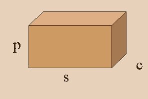
The TPC-D models a business warehouses, parts are bought from suppliers, and sold later to customers at a sale price. The database has information about each transaction for over a period of 6 years. So, we have 3 dimensions of interest: part, supplier and customer. For each cell (p,s,c) in this 3-D Data Cube , we store the total sales of part p that was bought from supplier s and sold to customer c.
The user can perform many queries on this database, for example:
In this example we compute the value of (p,ALL,c) where we derive from 3-D to 2-D summing on all suppliers. R refers to the raw data. The queries corresponding to the different sets of cells, differ only in the GROUP-BY clause. Therefore we will use the grouping attributes to identify the query (also referred to as view).
There are several approaches for materialization:
- Materialize the whole data cube. For example: Essbase (Hyperion) -Best query time, lots of space overhead.
- Materialize nothing. For example: BusinessObjects
- Materialize some of the views (queries). For example: MetaCube (Informix).
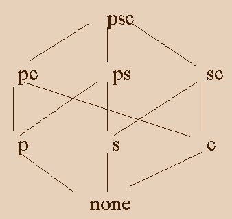
The Lattice Framework
We can define dependencies between queries (views). Since query (p,ALL,c) can be computed from (p,s,c) (summing on supplier), or (p,ALL,ALL) can be computed from (p,ALL,c) or (p,s,c) or (p,s,ALL) etc. So we can say that (p,ALL,ALL) is a descendent of the above mentioned queries, vice versa. (p,s,c) is the ancestor of (p,ALL,ALL).
The lattice is formed by the views
and their dependencies. A view corresponds to a vertex, and edges are formed
between immediate ancestor-descendent relation
(also referred to as next).
The framework also support hierarchies and composite lattices.
Example:
The Algorithm
The problem: Choosing k views from the set of all views.
Target: minimize the time of the queries.
This problem is NP-Complete (known reduction to set cover), so there isn't a known optimal algorithm (which runs in reasonable time). The article presents a greedy algorithm, which is proven to be within a known factor from the optimal.
Greedy algorithms (in concept) define some cost model on the data, and then choose from the data according to the cost (minimize or maximize). So, the first step in defining the algorithm is to establish the cost model:
The Cost Model
: The time to answer a query is taken to be equal to the space occupied by the view from which the query is answered. (It is actually linear in the space occupied by the query, but we can neglect that in the context of the algorithm).The Algorithm:
In each iteration we will compute the benefit of each view, and choose the one that gives us the most.
First, we'll define the benefit of each node:
suppose C(v) is the cost of view v. S is the lattice, we'll define B(v,S) to be:
In words: the effective benefit of
v in w will be according the views already in S,
and
will be the difference between what we could compute until now, and what we
would be able to do with the addition of v to S.
Then
the benefit of v will be the total benefit for all of it's descendents.
S = {top view};

for i = 1 to k begin

select that view v not is S
such that B(v,s) is maximized;

S = S union {v};

end;
The following example demonstrates the algorithm, the example shows a lattice of views and costs, and a table representing the calculation on the lattice:
The table:
Thus, the algorithm chose a (top view),b , f, d.
b was chosen since it improves the computation of b,d,e,g,h by 50 (from 100 of the view) and so on.
Results
The article presented the results
on the TPC-D benchmark, one can see the improvement in materializing some of the
view, and why materializing all views is not a good choice:
Conclusion and Future Work
Materialization of views is essential in order to minimize query time. It is an important optimization strategy (in addition to many other strategies).
Future work in this area can focus on:
In a similar article by the authors: Himanshu Gupta, Venky Harinarayan, Anand Rajaraman, Jeffrey D. Ullman, present a similar framework. The optimization in this article is on the views combined with indexes on the views. It is quite obvious that it is not efficient to scan a large view (even if was precomputed). The traditional approach is to select the views to precompute and on them select indexes. However, this is not the best approach, since they use the same space resource, and selecting a large view may force us to use small indexes. The article presents a family of algorithms of increasing time complexities.
The family of algorithms are greedy, and as always define a cost model on the views and queries (with a query - view graph). The family of algorithms are called: r-greedy.
Thus in 1-greedy algorithm we select in each iteration one object (view or index), in 2-greedy we examine all pairs and their contribution and select the pair that provide the best cost. Similarly r-greedy examine in each iteration r object together.
The complexity of the algorithms
are: ![]() . The larger
the r the solution is closer to optimal (and it takes more time to run the
algorithm). In the article they present experimental results on the TPC-D
database that show that for r=4 the results graph have a knee (meaning for r
> 4 there is a small increase in efficiency).
. The larger
the r the solution is closer to optimal (and it takes more time to run the
algorithm). In the article they present experimental results on the TPC-D
database that show that for r=4 the results graph have a knee (meaning for r
> 4 there is a small increase in efficiency).
My Summary:
The articles presented incorporate
databases with graphs and greedy algorithms. One can change the definition of
the problem to many other fields, since in the whole this is an approximation
problem (of an NP - complete problem).
The articles
present an initial framework, that need to be improved (like optimizing the
space constraint- with that approximating another NP-complete problem).
The article did not solve:
- Dynamicupdate of the database.
-
The selection of the views is static, it may be that during the life of the
database the views change, and materializing another view is essential.
This is yet another tool in the
ongoing straggle against the query time on data
warehouses.
I find it very elegant although it does
not give a full answer to the actual (real world) demands.