Decision Tree Building Algorithms
Classification is an important problem in data mining. The input to a
classifier is a training set of records, each of which is tagged with a class
label. A set of attribute values defines each record. The goal is to induce a
model or description for each class in terms of the attribute. The model is then
used to classify future records. The table below shows an example training set.
Classification has been successfully applied to several areas. Among the
techniques developed for classification, popular ones include bayesian
classification, neural networks, genetic algorithms and decision trees. In this
paper the focus is on decision trees. A decision tree is easily interpreted by
humans; inducing decision trees is efficient and is thus suitable for large
training sets; inducing decision trees do not require additional information
like domain knowledge or prior knowledge of distributions; Decision trees
display good classification accuracy.
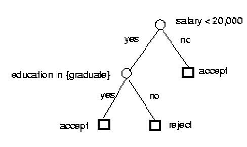
Below is a decision tree for the training data in the table. Each internal node
of the decision tree has a test involving an attribute, and an outgoing branch
for each possible outcome. Each leaf has an associated class. In order to
classify new records using a decision tree, beginning with the root node,
successive internal nodes are visited until a leaf is reached. At each internal
node, the test for the node is applied to the record. The class for the record
is simply the class of the final leaf node.
| salary | education | label |
| 10,000 | high-school | reject |
| 40,000 | under-graduate | accept |
| 15,000 | under-graduate | reject |
| 75,000 | graduate | accept |
| 18,000 | graduate | accept |
A number of algorithms for inducing decision trees have been proposed over the years. Most of them have two distinct phases, a building phase followed by a pruning phase. In the building phase, the training data set is recursively partitioned until all the records in a partition have the same class, and the leaf corresponding to it is labeled with the class. For every partition, a new node is added to the decision tree. The building phase constructs a perfect tree that accurately classifies every record from the training set. However, one often achieves greater accuracy in the classification of new objects by using an imperfect, smaller decision tree rather than one which perfectly classifies all known records. The reason is that a decision tree which is perfect for the known records may be overly sensitive to statistical irregularities and idiosyncrasies of the training set. Thus, most algorithms perform a pruning phase after the building phase in which nodes are iteratively pruned to prevent "overfitting".
The building phase for the various decision tree generation systems differs in the algorithm employed for selecting the test criterion for partitioning a set of records. The pruning phase differs mainly in the cost-complexity methods applied.
This section focuses on the building and pruning phases of a decision tree classifier, based on SPRINT in the building phase and on MDL in the pruning phase:
The tree is built breadth-first by recursively partitioning the data until
each partition contains records belonging to the same class. The splitting
condition for partitioning the data is either of the form ![]() if A is a numeric attribute or
if A is a numeric attribute or ![]() if A is a categorical attribute. For a set of records S, the entropy
if A is a categorical attribute. For a set of records S, the entropy![]() , where
, where ![]() is the
relative frequency of class j in S. Thus, the more homogeneous a set is with
respect to the classes of records in the set, the lower is its entropy. The
entropy of a split that divides S with n records into sets S1 with n1 records
and S2 with n2 records is
is the
relative frequency of class j in S. Thus, the more homogeneous a set is with
respect to the classes of records in the set, the lower is its entropy. The
entropy of a split that divides S with n records into sets S1 with n1 records
and S2 with n2 records is 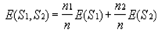 .
Consequently, the split with the least entropy best separates classes, and is
thus chosen as the best split for a node.
.
Consequently, the split with the least entropy best separates classes, and is
thus chosen as the best split for a node.
To prevent overfitting, the MDL principle is applied to prune the tree built
in the building phase and make it more general. The MDL principle states that
the "best" tree is the one that can be encoded using the fewest number
of bits. Thus, the challenge for the pruning phase is to find the subtree of the
tree that can be encoded with the least number of bits. In order to achieve
that, a scheme for encoding decision trees shall first be set. Then a pruning
algorithm may be set which, in the context of the encoding scheme, finds the
minimum cost subtree of the tree constructed in the building phase.
The cost of encoding the classes for n records, ni records in class i, may
be taken to be 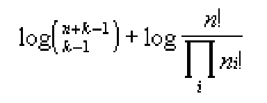
The cost of encoding the tree comprises of three separate costs:
The structure of the tree may be encoded by using a single bit in order to
specify whether a node of the tree is an internal node or leaf. The cost of
encoding each split involves specifying the attribute that is used to split the
node and the value for the attribute. The cost of encoding the data records in
each leaf was described above.
Using this scheme, the minimum cost subtree may be computed by a simple
recursive algorithm.
In most decision tree algorithms, a substantial effort is "wasted" in the building phase on growing portions of the tree that are subsequently pruned in the pruning phase. Consequently, if during the building phase, it were possible to "know" that a certain node is definitely going to be pruned, then it won't be expanded, and thus avoid the computational and I/O overhead. This is the approach followed by the PUBLIC (PrUning and BuiLding Integrated in Classification) classification algorithm that combines the pruning phase with the building phase.
The PUBLIC algorithm is similar to the SPRINT build procedure. The only difference is that periodically or after a certain number of nodes are split, the partially built tree is pruned. The MDL pruning algorithm represented cannot be used to prune the partial tree since the cost of the cheapest subtree rooted at a leaf in not known. This is because the tree is only partially built. Applying the algorithm as is will result in over-pruning.
In order to remedy the above problem, the MDL algorithm is used, while under-estimating the minimum cost of subtrees rooted at leaf nods that can still be expanded. With an under-estimate of the minimum subtree cost at nodes, the nodes pruned are a subset of those that would have been pruned anyway during the pruning phase. The PUBLIC algorithm distinguishes among three kinds of leaf nodes: Those that still need to be expanded; those that are result of pruning; those that cannot be expanded any further. Only for the first kind a lower bound is used. In PUBLIC, this modified pruning algorithm is invoked from the build procedure periodically. Once the building phase ends, there are no leaf nodes belonging to the first kind. As a result, applying the modified pruning algorithm at the end of the building phase has the same effect as applying the original pruning algorithm and results in the same pruned tree.
The experiments were conducted on real-life as well as synthetic data sets.
SPRINT is experimented as traditionally classification, against the PUBLIC(1),
PUBLIC(S) and PUBLIC(V) algorithms.
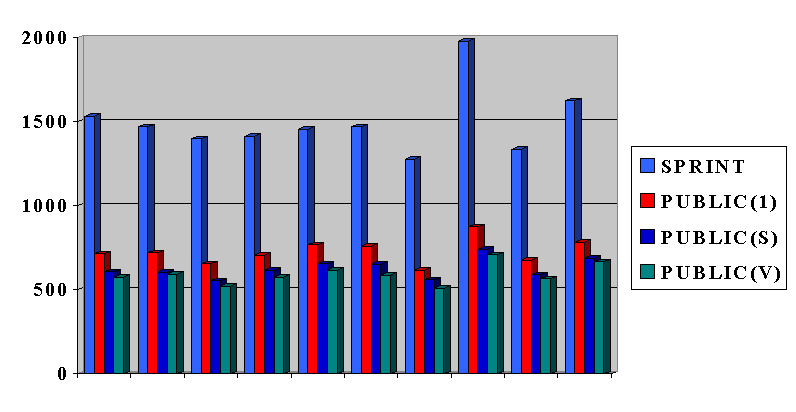
The experiments on the different real-life data sets are summarized in the
following graph, where the y axis indicates the time (in sec.).
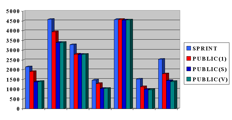
Generally, SPRINT takes between one to 83% more then the best PUBLIC algorithm.
The results for the synthetic data sets are given in the following graph:
Generally, SPRINT taken between 236% and 279% more then the best PUBLIC algorithm.
In my opinion, the publication clearly presents a simple idea for improving the complexity of inducing decision tree classifiers. The actual results are "proved" experimentally, which seems to suffice.
Alas, I've found myself dealing with some open issues in the paper: