Join Algorithms For Online Aggregation
.By Peter J. Haas and Joseph M. Hellerstein.
Summarized: Michal Ozery.
Introduction:
This paper presents a new family of join algorithms, called ripple joins, for online processing aggregation queries in a relational DBMS. Examples to aggregation operators are SUM, COUNT, AVG, STDEV, etc. As it is well known, traditional offline join algorithms are designed to minimize the time till completion. However, ripple joins are designed to minimize the time till an acceptably precise estimate of the query result is available. This time is independent in the size of the input relations. Since large-scale aggregation queries are typically used to get a "big picture" of data set, ripple joins' approach seem to be more attractive to use.
Current Systems process queries in "blocking" mode, meaning - no feedback till termination of the query. On the contrast, the output of ripple joins is continuously displayed to the user. The output of ripple joins is a series of progressively refined "confidence intervals" of the form [X
n - hn, Xn - hn] with a fixed probability p. Ripple joins are adaptive, adjusting their behavior in accordance with the statistical properties of the data. Moreover, they permit the user to tradeoff the time between successive updates of the confidence interval and the amount by which the confidence interval length (2*hn) decreases. Naturally, the longer the time between updates - the bigger the decrease in confidence interval length.
Assumption
: all the tupples of the input relations are processed in a random order.Overview of Ripple Join.
The main idea of ripple join is based on sampling. Since all the tuples are assumed to be randomly ordered, retrieving a new tuple can be considered as a sampling step. After each sampling step, the statistics are updated and the interval confidence is calculated.
In the simplest version of two-table ripple join, one previously-unseen random tuple is retrieved from each R and S at each sampling step. These new tuples are joined with the previousely-seen tuples and with each other. Thus the Cartesian product R x S is swept out as depicted in Figure 1.

Figure 1: The element of R x S that have been seen after n sampling steps of "square" ripple join (n = 1,2,3,4).
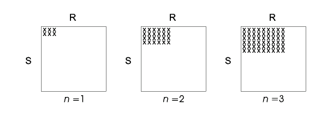
The "square" version of the ripple join described above draws samples from R and S at the same rate. However, in order to provide the shortest possible confidence intervals, it is often necessary to sample one relation at a higher rate than another. This requirement leads to the general "rectangular" version of the ripple join as depicted in Figure 2.

Figure 2: The element of R x S that have been seen after n sampling steps of "rectangular" ripple join (b
1 = 3, b2 = 2, n = 1,2,3).The general algorithm with K (>= 2) base relations R
1,…,RK retrieves bi previously-unseen random tuples from Ri at each sampling step for 1 <=i <= K. The sampling rates of the relations are called "aspect ratios". (Figure 3 corresponds to the special case in which K=2, b1=3, b2=2.) Note that when b1 = 1, bi = |Ri| the result is the known join algorithm "Nested Loops".Variations of Ripple Join.
Calculation of Confidence Intervals.
The computation of the confidence interval is based upon the Central Limit Theorem. The series of sampling steps can be considered as a series of independent, equally distributed random variables.
After each sampling step, the confidence interval (X
n+hn, Xn-hn) has to be updated. The estimation of the final result, Xn, is based on the sample set with the assumption of uniforimity on the complete Cartesian Product. (E.g. if we sampled .001 of the Cartesian Product and we calculated SUM=x, then Xn=1000 * x.).The confidence interval length h
n is estimated by a linear combination of the variances of statistical "data points" computed over the input Relations. Those "data points" are the values of conditional random variables {X[Ri,r], 1<=1<=K}; A conditional random variable X[R,r] is the result of the join condition of the Cartesian Product reduced to {r} on relation R (e.g. S x {r} instead of S x R). Since X[R,r] can't be computed without sweeping all relations except R - it is approximated in the same manner Xn is estimated.Adaptation of Ripple Join.
Obviously, the bigger the aspect ratios are - the longer it take to update the interval confidence (larger sample set). However, formulas show that h
n becomes shorter as the aspect ratios grow. Therefor, we have reached an optimization problem: minimizing hn while keeping the update time short as defined by the user. After each sampling step, the statistical properties of the data are updated causing hn to be updated as well. Thus every sampling step we have a new optimization problem followed by a new optimal values for aspect ratios.Personal Notes
(By Michal Ozery)