A Finite Sample Minimaxity Study of Model Selection Procedures based on
FDR control
Yoav Benjamini and Yulia Gavrilov[1]
Technical Report
Department of Statistics and Operations Research
Tel Aviv University
Abstract
The use of False Discovery Rate (FDR) controlling
procedure in model selection, in the form of penalized residual sum of squares,
is asymptotically minimax for  loss,
simultaneously throughout a range of sparsity classes for an orthogonal design
matrix (Abromovich et al 2000). In this work we discuss the finite sample
performance of such variable selection procedures as well as others that are
based on penalty based versions of FDR controlling procedures. We show by a
simulation study that the FDR controlling procedures have minimax performance
in this setting as well. We do that by comparing the performances of competing
model selection procedures on different data sets, with the reference
performance being that of a newly defined “random oracle” – the oracle model selection
performance on data dependent nested family of potential models. At the range
of configurations studied, 20-160 potential variables two methods performed
well: Tibshirani-Knight based penalty and Benjamini-Krieger-Yekutieli multiple
stages FDR testing based penalty. The latter is somewhat better for the largest
problems. Further gain is possible if the FDR level is adjusted to the problem
size and the correlation structure of the explanatory variables. Fixed penalty
per parameter methods such as Forward Selection, Cp (or AIC) perform poorly
even at these not too big problem sizes.
loss,
simultaneously throughout a range of sparsity classes for an orthogonal design
matrix (Abromovich et al 2000). In this work we discuss the finite sample
performance of such variable selection procedures as well as others that are
based on penalty based versions of FDR controlling procedures. We show by a
simulation study that the FDR controlling procedures have minimax performance
in this setting as well. We do that by comparing the performances of competing
model selection procedures on different data sets, with the reference
performance being that of a newly defined “random oracle” – the oracle model selection
performance on data dependent nested family of potential models. At the range
of configurations studied, 20-160 potential variables two methods performed
well: Tibshirani-Knight based penalty and Benjamini-Krieger-Yekutieli multiple
stages FDR testing based penalty. The latter is somewhat better for the largest
problems. Further gain is possible if the FDR level is adjusted to the problem
size and the correlation structure of the explanatory variables. Fixed penalty
per parameter methods such as Forward Selection, Cp (or AIC) perform poorly
even at these not too big problem sizes.
1. Introduction
The problem of variable selection has attracted the attention of both
applied and theoretical statisticians for a long time. Consider the widely used
linear model, ![]() , where Y is
a response variable,
, where Y is
a response variable,![]() is an n×m
matrix of potential explanatory variables,
is an n×m
matrix of potential explanatory variables, ![]() is a vector of unknown coefficients
(some coefficients may equal zero), and
is a vector of unknown coefficients
(some coefficients may equal zero), and ![]() is a random error. We want to select an
appropriate subset from the collection of the above m explanatory
variables in order to predict linearly the response variable. Selecting such a
subset is a difficult task: either too large or too small subset leads to a
large prediction error. The difficulty has tremendously increased with the
increasing size of the pool of explanatory variables encountered in recent
applications in data mining and bioinformatics.
is a random error. We want to select an
appropriate subset from the collection of the above m explanatory
variables in order to predict linearly the response variable. Selecting such a
subset is a difficult task: either too large or too small subset leads to a
large prediction error. The difficulty has tremendously increased with the
increasing size of the pool of explanatory variables encountered in recent
applications in data mining and bioinformatics.
There has been a wide range of contributions to solution of this
selection problem. To name a few of the most popular: Akaike’s information
criteria (AIC), which is motivated by using the expected Kullback-Leibler
information; Mallow’s Cp, which is based on the unbiased risk estimation;
Forward Selection and Backward Elimination which are based on hypotheses
testing and so on. Many of these selection criteria can be described as
choosing an appropriate subset of variables by adding a penalty function to the
loss function we wish to minimize. They differ by the nature of the penalizing
function, which is usually chosen to increase in the number of variables
already included in the model (see Miller 1990 for a comprehensive summary of
various traditional selection procedures).
The above four
examples share the same form of penalty function. The appropriate subset is
chosen by minimizing a model selection criterion of the form:![]() , where
, where![]() is the residual sum
of squares for a model with k=|S| parameters and λ is the penalization parameter. The first
two use λ=2, and the last two λ= z2a/2. Furthermore, the first two look for a
global minimum while the second two search for the first and last minima
respectively. An important common feature, though, is that the penalty per
additional parameter λ is fixed.
is the residual sum
of squares for a model with k=|S| parameters and λ is the penalization parameter. The first
two use λ=2, and the last two λ= z2a/2. Furthermore, the first two look for a
global minimum while the second two search for the first and last minima
respectively. An important common feature, though, is that the penalty per
additional parameter λ is fixed.
It has recently
been shown, in practice as well as theory, that variable selection procedures
with a fixed (nonadaptive) penalty are not effective when the real model size
can vary widely, which is the case when the problem is large in the sense that
potential number of explanatory variables is large (Shen and Ye (2002), George
and Foster (1997)). Procedures that perform well in one situation may perform
poorly in other situations. For instance, a large penalty per each parameter
entered into the model is likely to perform well when the size of the true
model is small or the true model has a parsimonious representation, but will
fail when most variables should be handled. For the last case small penalty is
appropriate but it is likely to give rise to many variables spuriously included
when the true model is small. In summary, for large problems, we need an
adaptive variable selection procedure that performs well across a variety of
situations.
Interestingly model selection
can be viewed as multiple hypotheses testing problem, in the sense that a
variable that is included in a linear model has a non zero coefficient , while a variable that is dropped has a zero
coefficient. It is natural to address such a decision using hypotheses testing
approach, and in fact in the orthogonal design case the fixed penalty per
parameter is equivalent to testing at some fixed level alpha of each
coefficient. Viewing our task as a multiple testing problem, we have to face
with the problem caused by the multiplicity of the errors that have to be
controlled simultaneously. The most familiar approach is Bonferroni that controls
the probability of rejecting any null hypotheses erroneously. The control of
such a stringent criterion leads to too few predictors entering the model. At
the other extreme lies the strategy to ignore the multiplicity issue
altogether, and test each hypotheses at level α.
, while a variable that is dropped has a zero
coefficient. It is natural to address such a decision using hypotheses testing
approach, and in fact in the orthogonal design case the fixed penalty per
parameter is equivalent to testing at some fixed level alpha of each
coefficient. Viewing our task as a multiple testing problem, we have to face
with the problem caused by the multiplicity of the errors that have to be
controlled simultaneously. The most familiar approach is Bonferroni that controls
the probability of rejecting any null hypotheses erroneously. The control of
such a stringent criterion leads to too few predictors entering the model. At
the other extreme lies the strategy to ignore the multiplicity issue
altogether, and test each hypotheses at level α.
We discuss a new criterion for
variable selection, based on controlling the False Discovery Rate (FDR) that
was advocated in Abramovich et al, 2000, hereafter ABDJ. FDR control is a
relatively recent innovation in simultaneous testing, defined as the expected
proportion of true null hypotheses rejected out of the total number of null
hypotheses rejected (Benjamini and Hochberg, 1995, hereafter BH). For an orthogonal design matrix it has
been show that the linear step-up FDR controlling procedure in BH is
asymptotically minimax for  loss,
simultaneously throughout a range of sparsity classes– (ABDJ). This FDR
controlling procedure is data adaptive, easy to implement, and as ABDJ show can
be phrased via a penalty function. The penalty per parameter increases with the
size of the problem, and for a given problem size the penalty is highest when
the true model contains no variables and smallest when the true model contains
all potential variables.
loss,
simultaneously throughout a range of sparsity classes– (ABDJ). This FDR
controlling procedure is data adaptive, easy to implement, and as ABDJ show can
be phrased via a penalty function. The penalty per parameter increases with the
size of the problem, and for a given problem size the penalty is highest when
the true model contains no variables and smallest when the true model contains
all potential variables.
The purpose of this modest work
is to check by a simulation study two additional aspects. First, whether the
conclusions of ABDJ are also valid for (i) non-orthogonal design matrices (ii)
models of finite size (iii) Non-sparse true models, in the sense that they may
include a large fraction of the potential variables (and even all). Second,
under the above conditions, to check whether newer adaptive FDR controlling
procedures offer further advantage over the BH procedure.
The asymptotic analysis of
Donoho and Johnstone (1994) used an oracle as a benchmark for comparing the
performance of competing methods. The question of the benchmark for comparison
of performance is more difficult in finite setting and for non-orthogonal
designs. We discuss (in Section 3) some options, and in particular choose to
compare the performance of the model selection procedures considered here to
the performance of an “oracle”. We do that by conditioning over the nested
sequence of models derived from a forward selection procedure used exhaustively
(with no penalty), and evaluating the optimal size of a model over this data
dependent sequence. This “random oracle” is our benchmark for comparisons and
minimaxity evaluation.
In the
next section we review non-constant penalized model selection methods that have
emerged in recent years including the adaptive FDR controlling methods from
Benjamini et al (2001) as much needed alternative to the fixed penalty methods.
In Section 4 we describe the simulation study and the results are reported and
analyzed in Section 5. We end by two applications of the leading competitors to
a Quantitative Trait Locus analysis in search for a modifier gene, and the
prediction of infant weight on birth, and a discussion of the implications of
this study.
2.
Model
Selection Procedure With Non-Constant Penalty
As we mentioned before, most of the penalized variable selection
procedures share the same form of penalty function and differ only by the value
of penalization coefficient, λ. They can be divided into three groups:
constant λ, λ that is the function of the size of the set
of variables over which the model is searched ![]() , and λ that is a function of both m and the
size of the model (k )
, and λ that is a function of both m and the
size of the model (k ) ![]() .
.
More traditional variable selection procedures choose the appropriate
subset by using the constant λ
(AIC, BIC). Donoho and Jonhstone (1994) suggested using 2log(m) as the
universal threshold leading to![]() . As noted before, the constant λ may be interpreted as a fixed level
testing. For example, AIC and Cp procedures, that use λ=2, are equal to test each hypothesis at
level 0.16. Donoho and Jonhstone threshold can also be viewed as a multiple
testing Bonferroni procedure at the level
. As noted before, the constant λ may be interpreted as a fixed level
testing. For example, AIC and Cp procedures, that use λ=2, are equal to test each hypothesis at
level 0.16. Donoho and Jonhstone threshold can also be viewed as a multiple
testing Bonferroni procedure at the level ![]() i. e.
i. e.![]() . Note that
. Note that![]() , when
, when![]() .
.
2.1 The BH
based penalty
ABDJ presented the
following FDR controlling procedure in a penalized form with a variable penalty
per parameter.
Associated with ![]() is its p-value,
is its p-value, ![]() and
and ![]() ordered according to their size p-values.
The linear step-up procedure in BH runs as follows:
ordered according to their size p-values.
The linear step-up procedure in BH runs as follows:
1.
Let ![]()
2.
If such a k
exists, reject the k hypotheses associated with ![]() . If no such k
exists, then none of the hypotheses is rejected.
. If no such k
exists, then none of the hypotheses is rejected.
This FDR procedure can be approximated by a
penalized method with a variable penalty factor ![]() . The procedure
itself exactly corresponds to the largest local minimum with the above penalty.
. The procedure
itself exactly corresponds to the largest local minimum with the above penalty.
The FDR parameter q plays an essential role in asymptotic
minimaxity theory in ABDJ. Even if we allow qm for problem of size m, but in such a way that qm→q<1/2, when m→∞, then it is sufficient for asymptotic
minimaxity. In contrast, if the limit q>1/2 asymptotic minimaxity is
prevented.
It is interesting to note that by for large m and k=o(m) the BH
penalty can be approximated by 2log(2m/qk) penalty, penalties of the
form that will be discussed in 2.3.
2.2
Other FDR based penalties
Building upon the
penalized approach to the BH multiple testing procedure in ABDJ, we present
here various other FDR testing procedures, and their approximation by a
penalized form. When the test statistics are independent or have positive
regression dependency the BH procedure controls the FDR at level ![]() , where
, where ![]() is an unknown number of true null
hypotheses. Of course, if
is an unknown number of true null
hypotheses. Of course, if ![]() is known, then q can be replaced
by
is known, then q can be replaced
by ![]() , and the FDR of the
above procedure at level q' is exactly at the right level q. This
motivates two-stage procedures, where at the first stage the value of
, and the FDR of the
above procedure at level q' is exactly at the right level q. This
motivates two-stage procedures, where at the first stage the value of ![]() is estimated and at the second stage
utilizes the estimates in the BH. One such two-stage procedure, suggested by
Benjamini, Krieger and Yekutieli (2001) can be described as follows:
is estimated and at the second stage
utilizes the estimates in the BH. One such two-stage procedure, suggested by
Benjamini, Krieger and Yekutieli (2001) can be described as follows:
1.
Use the BH
procedure at level q′=q/(1+q). Let ![]() be the number of rejected hypotheses. If
be the number of rejected hypotheses. If ![]() reject no
hypotheses and stop. If
reject no
hypotheses and stop. If ![]() reject all m
hypotheses and stop; otherwise
reject all m
hypotheses and stop; otherwise
2.
Let ![]()
3.
Use the linear
step up procedure at level ![]() .
.
This two-stage
procedure controls the FDR at the desired level q. A slight modification
where q is used at stage one and q′=q/(1+q) in stage two only,
was shown by a simulation study to control the FDR at level q as well.
Both versions were shown in the same simulation study to control the FDR for
positively correlated test statistics.
This testing
procedure can be approximated by minimizing twice BH penalized functions, once
with q and once with the data
dependent q*. It cannot be simply approximated by a
single penalty function.
The above two-stage procedure has been generalized by Benjamini, Krieger
and Yekutieli (2001) to a multiple stage procedure that can be described as the
step-down procedure as follows:
1.
Let ![]()
2.
If such a k
exists, reject the k hypotheses associated with ![]() ; otherwise reject
no hypothesis.
; otherwise reject
no hypothesis.
The multiple stage FDR procedure can be approximated by a penalized
method with the following variable penalty factor  .
.
Note, that in two
and multiple stage procedures the hypotheses can be rejected even if its p-value
is greater than 0.5, or in extreme cases for whatever its value is. This is not
surprising, since all the hypotheses are tested simultaneously and the control
of FDR allows a few erroneous rejections if many correct rejections have
already been made. If there are situations where one does not want to reject
those hypotheses with large p-values, he may simply add the constraint
that the hypotheses cannot be rejected if the corresponding p-value is
larger than some prespecified value, leading to  .
.
2.3
Other non-constant penalties
Several independent groups of researchers have recently proposed model
selection rules with penalty factors that is function of both m and k:
1.
Foster and
Stine (1997) arrived at a penalty ![]() from information theoretic
considerations.
from information theoretic
considerations.
2.
Tibshirani and
Knight (1999) propose model selection using a covariance inflation criterion
that adjusts the training error by the average covariance of predictions and
responses on permuted versions of dataset. In the case of orthogonal
regression, their proposal takes the form of complexity penalized residual sum
of squares, with the complexity penalty approximately of the above form, but
larger by a factor of 2: ![]() .
.
3.
Birgé and
Massart have studied complexity penalized model selection for a large class of
penalty functions, specifically designed to include penalties of the form ![]() . They develop
non-asymptotic risk bounds for such procedures over
. They develop
non-asymptotic risk bounds for such procedures over ![]() balls.
balls.
4.
Finally,
George and Foster (1997) adopt an empirical Bayes approach, drawing the
components from a mixture prior ![]() and then estimating the hyperparameters
(w, C) from the data. They argue that the resulting estimator penalizes the
addition of a kth variable by a quantity close to
and then estimating the hyperparameters
(w, C) from the data. They argue that the resulting estimator penalizes the
addition of a kth variable by a quantity close to ![]() .
.
2.4 Search strategy
In principle, in order to get an appropriate subset of variables by some
strategy, we should check all![]() candidate models
and choose the subset that minimizes the sum of the RSS and the penalty.
In problems of even medium size it is technically impossible to apply such
exhaustive search. For example, the upper computational limits are m≤30
in Splus and m≤100 in SAS. Another possibility is to select the best
model over a backward or forward path of nested models. Such a path is data
dependent and may be constructed using a greedy algorithm. Although the
collection of models along the “forward/backward path” need not contain the
best overall one, it is practically been the most common way this problem in
handled. Note that if the design matrix is orthogonal the paths generated by
the forward selection and the backward elimination is the same. Once the design
matrix is non-orthogonal, these two may yield different paths. Having in mind
current large applications where the number of variable considered may be
larger than the number of observations available, we adhere in this work to the
path generated by forward selection.
The result is a random (data dependent) path of nested models of size k,
k=1,2,..,m. All penalized procedures search for a global minimum of the
penalized loss on this sequence.
candidate models
and choose the subset that minimizes the sum of the RSS and the penalty.
In problems of even medium size it is technically impossible to apply such
exhaustive search. For example, the upper computational limits are m≤30
in Splus and m≤100 in SAS. Another possibility is to select the best
model over a backward or forward path of nested models. Such a path is data
dependent and may be constructed using a greedy algorithm. Although the
collection of models along the “forward/backward path” need not contain the
best overall one, it is practically been the most common way this problem in
handled. Note that if the design matrix is orthogonal the paths generated by
the forward selection and the backward elimination is the same. Once the design
matrix is non-orthogonal, these two may yield different paths. Having in mind
current large applications where the number of variable considered may be
larger than the number of observations available, we adhere in this work to the
path generated by forward selection.
The result is a random (data dependent) path of nested models of size k,
k=1,2,..,m. All penalized procedures search for a global minimum of the
penalized loss on this sequence.
Forward selection and backward elimination may also differ in the
resulting model even when they produce the same path, because they have
different stopping rules that stem from the different directions of search.
Only if ![]() or constant we get the same solution by both forward and backward search, a
solution that is also the global minimum.
For the adaptive penalty coefficients
or constant we get the same solution by both forward and backward search, a
solution that is also the global minimum.
For the adaptive penalty coefficients ![]() the three need
not coincide even in the orthogonal case.
the three need
not coincide even in the orthogonal case.
Regarding the BH procedure in its penalized form, it was shown by ABDJ
that for the orthogonal design matrix the difference between the locations of
rightmost minimum (the backward elimination solution) and leftmost local minimum
(the forward selection solution) is uniformly small enough on sparse spaces.
The rightmost minimum corresponds to the BH, the leftmost minimum corresponds
to a testing procedure that also controls the FDR (Sarkar, 2002). Therefore the
asymptotic minimaxity of the global minimum holds for the other two as well.
Moreover, by their numerical results these indices are often identical.
We shall use a similar approach with the new FDR testing based
penalties, searching for the global minimum rather then by the direction
indicated by the testing procedure.
3. The Comparisons Between
Different Selection Procedures
To make a fair comparison between different selection procedures we use σ =1 for all of the procedures so that we can
separate the task of variable selection from that of estimating the unknown σ.
For each configuration of parameters (the configurations will be defined
in section 4.2) the goodness of fit of each estimator was measured by its mean
square predicted error ![]() . In order to
compare estimators across different configurations the relative errors have to
be defined in order to neutralize the configuration’s effect and enable us to
compare the wide range of the situations. Note, that for each configuration
separately, an estimator that minimizes the MSPE minimizes also the relative
error.
. In order to
compare estimators across different configurations the relative errors have to
be defined in order to neutralize the configuration’s effect and enable us to
compare the wide range of the situations. Note, that for each configuration
separately, an estimator that minimizes the MSPE minimizes also the relative
error.
Since in a real dataset the
configuration of parameters is unknown, we would like to find the variable
selection procedure whose maximum relative MSPE is minimal over a wide range of
configurations, i.e. the method that is the minimax solution.
There are several possibilities to define the base against which the
relative error is evaluated.
1.
Real Model
In a simulation study the subset of true predictors and their effects
are known, therefore we can build the true model and compute its mean square
predicted error that will be noted as ![]() . Then the relative
MSPE for each estimator is evaluated as
. Then the relative
MSPE for each estimator is evaluated as ![]() .
.
2.
Oracle
Model
The second way to find the best estimator is to compare each MSPE with
theoretical minimal MSPE. The estimators of the coefficients that are based on
the real model are unbiased and its MSPE is composed only of the variance term.
By deleting some explanatory variables whose coefficients are very small but
not zero, we may be able to get a biased model that enjoys smaller MSPE. The
best such model is defined as an oracle model and its mean square predicted
error will be noted as ![]() .
.
For orthogonal vector of parameters the ideal risk (that is defined as ℓ2-loss) is attained if only those parameters
that are larger than the noise level are estimated (Donoho and Jonhstone 1995). In our case it
means that the oracle model should consists only of those explanatory variables
for which absolute value of coefficient is larger than its noise level i.e.,![]() . For any finite model it can easily be shown that deleting a
true variable that does not satisfy the above condition decreases the MSPE.
. For any finite model it can easily be shown that deleting a
true variable that does not satisfy the above condition decreases the MSPE.
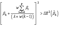
For dependent predictors we can imitate the above by applying the
following procedure: the first step for dependent predictors is equal to that
of orthogonal predictors, i.e., the variable with the smallest effect should be
dropped from the true model if its absolute value of coefficient is smaller than
the noise level. Further steps are more complicated because the model gets
bias. They still involve comparing the size of β with its
standard error but it also involves the correlation structure as well as the
size of the parameters that already left out. It can be shown that the k-th explanatory variable should be kept in
the model if: ![]() . In particular case where all correlations are equal we get
. In particular case where all correlations are equal we get![]() , where
, where ![]() and
and ![]() . Because of the dependency such a search does not necessary
produce the best possible subset of predictors, and at the same time may be
irrelevant for the purpose of performance comparisons.
. Because of the dependency such a search does not necessary
produce the best possible subset of predictors, and at the same time may be
irrelevant for the purpose of performance comparisons.
3.
Random
Oracle
Therefore, we turn
to defining the random oracle. As explained
above, it is practical to confine ourselves to using a stepwise search of forward selection.
While the stepwise search does not guarantee that the global optimizer is
located as one of the nested models, the performances of tested selection
procedures are beforehand restricted. Thus the oracle MSPE is still idealistic
a base value for a comparison with MSPE of other methods. In order to get a
more appropriate comparison we define an oracle on a sequence of nested models, where the sequence
exhausts all variables. The sequence may be random in the sense that it depends
on X and Y, as is the case when using forward selection. The random
oracle selects an appropriate
subset of variables along the path of nested models, but taking the values of
the real coefficients into account. Let us denote its performance by MSPEoracle(X,Y).
Then, we compare the performance of each procedure on the same random sequence
relative to the performance of the random oracle. This comparison is more
appropriate because it neutralizes the stochastic component in the comparison
that depends on the chosen sequence of nested models (a path in the model
space) and gives us a common basis for all procedures even if the chosen path
is far from optimal.
4.
Best Performer
We can also compare each MSPE with the best estimator among the tested
ones, i.e., the one achieving the minimum MSPE at that configuration. From this
point of view, the performance of i-th selection rule can be measured by
the ratio ![]() . The closer this
ratio to one, the better the estimator is. The deficiency of this approach is
that the results depend on specific selection procedures included in the study. If we chose some other procedures, we might get different
results and conclusions. In particular if we omitted a good procedure at some
configuration it might significantly change the ratio.
. The closer this
ratio to one, the better the estimator is. The deficiency of this approach is
that the results depend on specific selection procedures included in the study. If we chose some other procedures, we might get different
results and conclusions. In particular if we omitted a good procedure at some
configuration it might significantly change the ratio.
Note, that we give
two meanings for forward selection: we keep the term “forward selection” for
the procedure that selects the sequence of nested models (by series of ![]() z-tests if σ is known, F-tests if σ
is unknown) along with using fixed level testing to decide whether to enter one
more variable. We use the term “forward path selection” for the calculated
sequence of nested models generated by forward selection without testing.
Different selection procedures can select an appropriate model on this sequence
accordingly to their stopping rule.
z-tests if σ is known, F-tests if σ
is unknown) along with using fixed level testing to decide whether to enter one
more variable. We use the term “forward path selection” for the calculated
sequence of nested models generated by forward selection without testing.
Different selection procedures can select an appropriate model on this sequence
accordingly to their stopping rule.
4.
Simulation Study
A Simulation study was performed to compare the efficiency of the FDR
controlling procedures and some other selection rules.
4.1 The procedures
Ten model selection procedures were compared
with the random oracle and the true model performance:
1.
The Linear
Step-up procedure in BH - FDR
2.
The two-stage
FDR procedure (the modified version) in Benjamini, Krieger and Yekutieli -
TSFDR
3.
The
multiple-stage procedure in -
MSFDR
4.
Forward
selection procedure - FWD
5.
The procedure
in Foster and Stine (1997) - FS
6.
The procedure
in Tibshirani and Knight (1999)- TK
7.
The procedure
in Birgé and Massart (2001) - BM
8.
The procedure
in George and Foster (1997) - GF
9.
The universal
threshold in Donoho and Johnstone (1994) - DJ
10.
AIC (Cp)
procedure.
The first four procedures were implemented
at levels: 0.05,0.10, 0.25, 0.50, resulting in 22 model selection procedures.
4.2 The Configurations Investigated
Simulations are conducted with correlated and independent covariates. A
random sample ![]() is generated according to
is generated according to ![]() ,
, ![]() . The number of
potential explanatory variables, m is 20, 40, 80 and 160, the number of
real explanatory variables (with non-zero coefficients) is p=
. The number of
potential explanatory variables, m is 20, 40, 80 and 160, the number of
real explanatory variables (with non-zero coefficients) is p=![]() , m/4, m/3,
m/2, 3m/4, and m. The number of observations n is always
2m, and σ =1. For each m, three design matrices were generated for three
values of
, m/4, m/3,
m/2, 3m/4, and m. The number of observations n is always
2m, and σ =1. For each m, three design matrices were generated for three
values of ![]() , from
, from ![]() with
with ![]() whose diagonal elements are 1 and whose ijth
element is
whose diagonal elements are 1 and whose ijth
element is ![]() for
for ![]() . For each
configuration of the parameters defined above, three different choices of β are considered:
. For each
configuration of the parameters defined above, three different choices of β are considered:
(1) ![]() .
.
(2) ![]() for p=m/2,
for p=m/2, ![]() for p=m/3,
for p=m/3, ![]() for p=m/4,
for p=m/4, ![]() for p=3m/4 and
for p=3m/4 and ![]() for p=m, so the smallest
non zero
for p=m, so the smallest
non zero![]() will be always
will be always![]() . For p=√m
. For p=√m
![]() was chosen uniformly on the interval
was chosen uniformly on the interval ![]() (1/m, 1 ).
(1/m, 1 ).
Configuration (2) differs from configuration (1) both in the rate of
decrease and in the fact that the minimal ![]() is constant
across p. In both
configurations
is constant
across p. In both
configurations ![]() is chosen so that the standard error of
the least squares estimators of the coefficients in the true model will be
approximately equal for all values of m.
is chosen so that the standard error of
the least squares estimators of the coefficients in the true model will be
approximately equal for all values of m.
(3)![]() , where the value of
c(p) is chosen to give a theoretical
, where the value of
c(p) is chosen to give a theoretical ![]() . The value of c(p) decreases as p increases.
. The value of c(p) decreases as p increases.
Configuration (3) was chosen as it has been
used by several authors as a test case in their simulation studies. (George,
Foster, 2000; Shen, Ye, 2002). Therefore, it was interesting to include it in
the current study as well.
The intercept for all
configurations was chosen ![]() , so that it is
practically always included in the model.
, so that it is
practically always included in the model.
In our first simulation study (not reported here) five types of
coefficients with different ![]() factors were tested. The configurations of
coefficients presented here expose extreme performances for all compared
selection procedures to the better or the worse.
factors were tested. The configurations of
coefficients presented here expose extreme performances for all compared
selection procedures to the better or the worse.
4.3 Computational procedures
The performance of each model selection procedure in each configuration
was measured by its mean square predicted error averaged over 1000
replications. The computational task involved in the current study was beyond
achievement using a single computer within a reasonable time frame. We
therefore utilized the software tool for computer-intensive jobs, Condor (http://www.cs.wisc.edu/condor/), which allows running serially and in parallel
jobs, using the large collections of distributively owned computing resources.
In our case we used the approximately 80 computers in our Students Computer Lab
at the Schools of Computer Sciences and Mathematical Sciences at Tel Aviv
University (operating on LINUX).
Standard errors for the relative performance of each method to the
random oracle were approximated from standard errors of MSPE from the
simulation results, following (Cochran).
5. The Simulation Results
Figure 1 presents the MSPE values of all studied FDR procedures at levels 0.05, 0.10 and 0.25 relative to those of the random oracle estimator over all configurations for each m and ρ separately. Based on our simulation results, and as indicated by ABDJ, q=0.50 never leads to the best performances. Therefore, FDR procedures at level 0.50 are not presented in figure 1.
It can be seen from figure 1 that the FDR control parameter q
plays an important role in achieving the minimal loss in each specific
configuration studied. Take, for example, m=160, ρ=0, “Sqrt”. For configuration with “1” (![]() ), using q=0.05 is best for all FDR procedures, while
under the same setting for “6” (p=m) q=0.25 is the best.
As expected, the small values of q perform better in “small” models and
vice versa. However, the information available for the model builder is only on
m, sometimes on ρ,
rarely vaguely on p and never on the structure of the coefficients.
Therefore, if we choose q using a
minimax consideration over the last two we get table 1 that summarizes the
preferable values of q for the FDR procedures.
), using q=0.05 is best for all FDR procedures, while
under the same setting for “6” (p=m) q=0.25 is the best.
As expected, the small values of q perform better in “small” models and
vice versa. However, the information available for the model builder is only on
m, sometimes on ρ,
rarely vaguely on p and never on the structure of the coefficients.
Therefore, if we choose q using a
minimax consideration over the last two we get table 1 that summarizes the
preferable values of q for the FDR procedures.
Table 1:
The preferable values of q for tested FDR procedures.
|
|
|
BH |
TSFDR |
MSFDR |
|
m=20 and 40 |
ρ=-0.5 |
0.05 |
0.05 |
0.05 |
|
ρ=0 |
0.05 |
0.05 |
0.05 |
|
|
ρ=0.5 |
0.05 |
0.05 |
0.05 |
|
|
General correlation |
0.05 |
0.05 |
0.05 |
|
|
m=80 |
ρ=-0.5 |
0.1 |
0.1 |
0.1 |
|
ρ=0 |
0.1 |
0.05 |
0.05 |
|
|
ρ=0.5 |
0.1 |
0.05 |
0.05 |
|
|
General correlation |
0.1 |
0.1 |
0.05 |
|
|
m=160 |
ρ=-0.5 |
0.25 |
0.25 |
0.25/0.1 |
|
ρ=0 |
0.1 |
0.1 |
0.05 |
|
|
ρ=0.5 |
0.1 |
0.1 |
0.1 |
|
|
General correlation |
0.1 |
0.1 |
0.05 |
From this table it seems that the smaller values of q (0.05 and
0.1) perform better than q=0.25. In addition, while the optimal choice
of q for BH procedure varies across different m values, within the
same size m it varied only in the configuration ρ=-05.
For TSFDR procedure the
optimal values of q are more stable as m changes, and even more
so for the MSFDR procedure. The actual relative MSPE achieved by the two
methods are quite close to each other
BH procedure performs
better than adaptive FDR procedures
(two and multiple stage) only for “small” models, where meaning of “small”
depends on both p and m size. For example, p up to m/3
for m=20 and p up to ![]() for m=160.
Note that the relative loss of using the adaptive procedures instead of BH in
“small” models is less than the relative loss of using BH instead of adaptive
procedures in rich models. Therefore by minimax criterion we recommend to use
adaptive FDR procedures. The advantage of this using will be greater as bigger
the m and richer the model. Note that for all FDR procedures the
relative loss to random oracle is decreases as bigger the m, which means
that in the large problems (m=160 and above) the performances of FDR
procedures will be very close to those of the random oracle. The maximal loss
relatively to random oracle of BH procedure at 0.05 gets up to 1.72, 1.78, 1.98
and 1.87, of two stage FDR procedure at 0.05 gets up to 1.62, 1.74, 1.82 and
1.81, of multiple stage FDR procedure at 0.05 gets up to 1.47, 1.72, 1.77 and
1.79 for m=20, 40, 80, 160 respectively.
for m=160.
Note that the relative loss of using the adaptive procedures instead of BH in
“small” models is less than the relative loss of using BH instead of adaptive
procedures in rich models. Therefore by minimax criterion we recommend to use
adaptive FDR procedures. The advantage of this using will be greater as bigger
the m and richer the model. Note that for all FDR procedures the
relative loss to random oracle is decreases as bigger the m, which means
that in the large problems (m=160 and above) the performances of FDR
procedures will be very close to those of the random oracle. The maximal loss
relatively to random oracle of BH procedure at 0.05 gets up to 1.72, 1.78, 1.98
and 1.87, of two stage FDR procedure at 0.05 gets up to 1.62, 1.74, 1.82 and
1.81, of multiple stage FDR procedure at 0.05 gets up to 1.47, 1.72, 1.77 and
1.79 for m=20, 40, 80, 160 respectively.
Based on above, for the range of situations investigated here, if a
single FDR based model selection procedure should be recommended with a single
fixed q – we recommend the use of MSFDR at 0.05.
Table 2: the maximal mean MSPE values relative to those of the random
oracle (based on 1000 replications).
|
Procedure |
M=20 |
M=40 |
M=80 |
M=160 |
|
FWD |
2.80 (0.068) |
2.87 (0.061) |
2.84 (0.043) |
3.59 (0.098) |
|
Cp |
4.77 (0.096) |
4.87 (0.096) |
4.88 (0.069) |
6.88 (0.193) |
|
DJ |
2.34 (0.022) |
2.78 (0.021) |
3.05 (0.016) |
2.58 (0.010) |
|
BM |
4.47 (0.064) |
5.15 (0.106) |
6.61 (0.137) |
5.09 (0.110) |
|
FS |
3.07 (0.097) |
3.62 (0.090) |
3.35 (0.059) |
3.35 (0.068) |
|
TK |
1.66 (0.028) |
1.71 (0.015) |
1.72 (0.010) |
1.99 (0.010) |
|
MSFDR 0.05 |
1.47 (0.031) |
1.72 (0.012) |
1.77 (0.010) |
1.79 (0.008) |
The numbers in parentheses
are the corresponding standard errors of the relative loss (mean MSPE value of
each method divided by mean MSPE value of random oracle)
The numbers that are
emphasized by border are the minimal relative loss. The numbers in the gray
cells are in the range of one standard error from the minimal relative loss.
From this point of view the two leading procedures are MSFDR 0.05 and
the TK, each one achieving minimax performance for two problem sizes. Still,
comparing just these two, the inefficiency of the MSFDR relative to TK is
maximally 2.9%, while the other way around it is 12.9%., and for m=40
the two are hardly distinguishable.
The maximal relative loss by DJ procedure gets up 3.05 and is performing
better in our study than the other variable penalties that depend both on m
and p that reach 3.62 for FS and 6.61 for BM. Cp and FWD at 0.05 get up to 6.88 and 3.59, and further note
that the values in the table increase as m increase indicating the
increasing deterioration of performance for large problems. But even for our
small problems they do not perform well.
So far we have done the comparisons only utilizing the information about
m. If further information is available on the structure of the
dependency among the explanatory variables we may wish to look into the results
on the finer resolution. Figure 2 summarizes for each m and ρ separately the mean MSPE values relative to
those of the random oracle over the subset of configurations of interest as
discussed in Section 4.2. The results are presented for the selection
procedures discussed in Section 4.1, and the MSFDR at 0.05 as the single FDR
candidate.
The general result is quite similar to the one previously described in
the sense that MSFDR and the TK are always the minimax procedures, about half
“wins” for each. Generally, the MSFDR has the advantage for m=20 and m=160,
the TK for the other two, with very small differences for m=40. If we
further allow q to depend on m and ρ, then when the TK has the advantage the two
have similar performance and when the MSFDR takes the lead the TK is further
behind. The least favorable situations for both were usually the extreme models
either the smallest or the largest. The structure of the coefficients was
either a constant or decay as the square root.
The performance of the DJ
procedure is similar for all values of ρ. Large models strain its performance, as
can be expected. It performs better for sparse models although it is never the
best, as predicted by the asymptotic theory.
The performance of BM procedure was worse by minimax criterion compared
to above procedures with non-constant penalty, although in some situations this
procedure was the best among the tested ones. For example, for ρ=-0.5 and constant coefficients for m=20,
40 and 80 the performances of BM procedure were as good as those of random
oracle. Its maximal relative
loss occurs for the configurations where coefficients decay as a square root,
mostly for extreme size of true model: too sparse or too rich.
Performances of two methods (AIC, Forward selection) with fixed λ were systematically worse (by minimax
criterion) compared to the mentioned above adaptive penalties. These methods
perform better when the size of the true model is large, but for small model
sizes the loss relatively to the random oracle of using forward selection is
high.
GF procedures perform poorly (more than 20 fold) in spite of its
adaptive penalty (therefore this procedure is not presented at fig.2). This
happens because the penalty function of the method is not high enough for the
first variables that enter the model comparing to other adaptive procedures
studied here. In addition the penalty is not increasing monotonically, and
therefore yields overfitted models. The penalty of GF procedure starts to
decrease as the model includes more than m/2 variable. Thus, if m/2
explanatory variables get into the model, automatically we are bound to include
all variables.
6. Examples
6.1
Modifiers genes for the Bronx waltzer mutation
The experiment was conducted in order to identify the genetic factors
that influence the behavior and the hearing ability of the bv strain of
mice. This strain has a recessive mutation located in chromosome 5. By studying
the effect of other genes on the hearing ability via a linear regression model,
their modifying effect on the bv mutation can be assessed. Thus the
explanatory variables are the dummy variables representing the markers where
the information about each mouse genome is available. Such information was
available to us about 45 markers on 5 chromosomes only, but the selected
chromosomes were all those that exhibited markers with nominal significance (p<0.1)
in the initial statistical analysis conducted by investigators. All work with
the mice and the initial statistical analysis was performed in Karen P. Steel’s
laboratory.
Had there been no initial selection we could use the investigated model
selection procedure with m=45. We by-pass the difficulty assuming that
the number of initial tested markers on each chromosome was approximately the
same, so we set the total number of tested markers as m ≈ 45(19/5)=171.
It is known from the literature that there should be the positive correlation
between the markers at the same chromosome and no correlation between the
markers at the different chromosomes, so we can make use of the results of
simulation study for m=160 and ρ=0.5, and choose q=0.1 for all FDR
procedures. All other procedures were applied to these data.
Most of the variable penalty tested procedures yield the same results.
DJ, TK, FS and all FDR procedures found a single significant marker that is
located at chromosome 4 (D4Mit125). BM procedure did not find any significant
marker. In contrast the forward selection found an additional significant
marker at chromosome 9, and Cp found 13 significant markers that are scattered
over all 5 chromosomes. From another statistical analyses (Yakobov et al 2001)
it was found that there are two significant QTL regions, the first near
D4Mit168 and the second between D4Mit125 and D4Mit54 (both at chromosome 4).
Note, that there is a very strong positive correlation between the markers of
chromosome 4 (up to 0.98) which can explain the why a linear regression method
discovered one marker on chromosome 4 but not the other.
6.2 Prediction of infant weight at birth
The data of this example come from a study (Salomon et al., 2004). There
are 64 different potential explanatory variables such as personal
characteristics (weight, age, smoking, etc.), health status (diabetes,
hypertension, etc.), prothrombotic factors, and the results of the different
tests performed during the pregnancy (including their dates). The predictors
are such that we can make no assumption about the type of the dependency among
them we face.
Based on the simulation results for m=80 we choose q=0.1
for the linear step-up and two stage FDR procedure and q=0.05 for the
multiple stage FDR procedure. The Cp method resulted in 10 significant
predictors, the forward selection method in 7 significant explanatory
variables, FS - 5 significant ones, TK, DJ and BM procedures all found only 2
significant variables and all FDR procedures found 4 significant variables to
be included in the linear model. The predictors that were found by FDR
procedures are: the length of the pregnancy, the estimated embryo weight at the
second test, the mother’s weight when she was born and the variable indicating
whether cesarean section was planned or not. All of these are known from the
literature as good single predictors for infant weight at the birth. As it
turns from the analysis using all four together in the model turn out to
further improve prediction.
7.
Discussion
In summary, there are two procedures that
perform well in all tested situations – TK and the multiple stage FDR procedure
at level 0.05, an advantage to the MSFDR at large problems. In order to understand
the similarity and differences in the results for the TK and MSFDR procedures
over the studied range of configurations we plot the penalty per coefficient in
Figure 3. As evident from this figure, the penalty of the MSFDR procedure is
lower for the first variables that enter the model than the penalty of the TK,
and higher for the rest of the variables. The penalty of MSFDR begins like the
BH procedure and ends like the TK procedure.
For m=160 the worst performances of
both procedures are achieved at the same configuration for constant
coefficients. The oracle for this configuration leaves all variables in the
model. When the mean number of the predictors in the models by both procedures
is less than m/5.5 (about 30 variables) the performances of FDR procedures
are better than TK. In this range the FDR penalties are more lenient comparing
to the TK penalty and, therefore, enter more variables into the model, yielding
better prediction. Such configurations are generally least favorable for the TK
penalty and in these configurations an adaptive FDR procedures (two stage and
multiple stage) perform better than the linear step up procedure. When the mean
number of the predictors in the models by both procedures is more than m/5.5
we get an opposite situation, because in this range the TK penalties are more
lenient. When the mean number of the predictors in the models by both
procedures is about m/5.5 the performances are similar.
Tibshirani and Knight (1999) originally
suggested a complex procedure for model selection in the general, and the TK
penalty (used here) was developed as the equivalent for the orthogonal design
matrix. It is thus interesting to note that in most cases in our simulation the
performances of this penalty in correlated data were better than in the case of
ρ=0. The comparison with the actual
covariance estimation procedure remains to be seen, but we think that the much
simpler penalty based selection method will perform about the same, in minimax
sense.
As noted before
allowing dependency on q in the MSFDR is hardly a limitation since m is always known. The simulation study
in ABDJ for the orthogonal case studied the BH performance for m=1024
and 65536, and the recommended value was about q=0.4. It does seem that
the optimal q increases in m, but of course cannot exceed 0.5.
Since we got the
same value of q for optimality in the general case as in ρ=0, the above indication may hold promise
for the general case as well. The dependency of q on m, and
possibly on other factors known to the modeler, is an interesting research
problem that will benefit from further theoretical and empirical study.
A problem that has not been addressed in this article is the estimation of the standard deviation of the error. In real problems this parameter is usually unknown. Even though the statistical literature includes many proposals, the estimation is a real challenge when number of predictors is large, especially when it is larger than the number of observations.
Figure 1: MSPE
values relative to the random oracle of penalized FDR procedures: The
line type expresses the procedure, BH (–), TSFDR (….), MSFDR (![]() ) and the
symbol the level of FDR control 5% (○), 10% (∆) and 25% (+).
) and the
symbol the level of FDR control 5% (○), 10% (∆) and 25% (+).
Figure 2: MSPE values relative to the random
oracle: MSFDR (Δ), DJ (+), FS(×), BM )□), TK (○), FWD 5% (■), Cp (●).
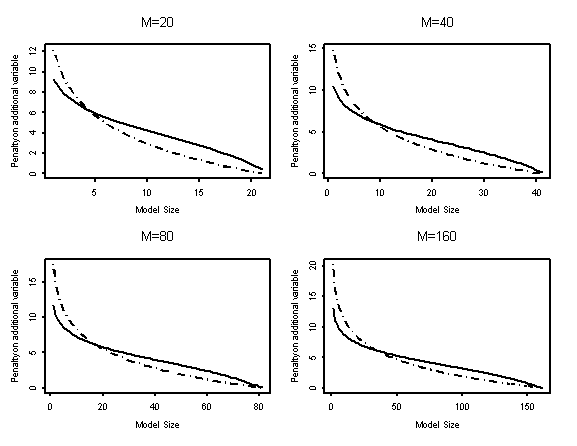
Figure 3: Comparing the Multiple Stage FDR and
the Tibshirani-Knight penalties at the studied problem sizes. The solid line
for MSFDR at 0.05 and the dotted line for TK procedure.
Appendix
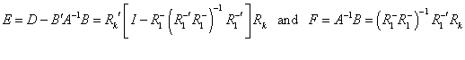
Let X be the nxp matrix of true explanatory variables. We can express X=ZR, where
R is the correlation matrix Z is an approximately orthogonal
matrix. Let ![]() , where
, where![]() ,
, ![]() ,
, ![]() ,
, ![]() are the correlation
matrices of k, (p-k), (k-1) and (p-k+1) variables
respectively. At the same way we can define the
are the correlation
matrices of k, (p-k), (k-1) and (p-k+1) variables
respectively. At the same way we can define the ![]() ,
, ![]() ,
, ![]() ,
, ![]() and the
and the![]() ,
, ![]() ,
, ![]() ,
, ![]() .
.
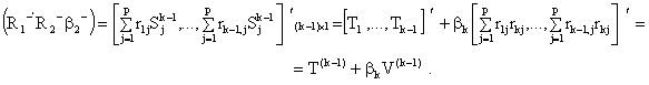
It is known that mean square predicted error
of model that consists of k variable is:
In a similar way,
![]()
Define,
![]() ,
,
and
![]() .
.
The difference between the first terms of ![]() and
and ![]() is:
is:
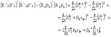
Now, define
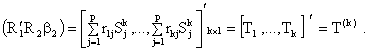
In the model with (k-1)
variables we get:
The second term in the
expression for the![]() is,
is,
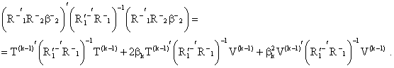
Expressing ![]() in terms of
in terms of ![]() we get
we get
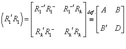 , where
 ![]() , whose inverse can be
written as
, whose inverse can be
written as
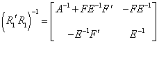 ,
,
 .
.
The second term in ![]() is
is
![]() .
.
Now, the difference between the
![]() and
and ![]() is:
is:
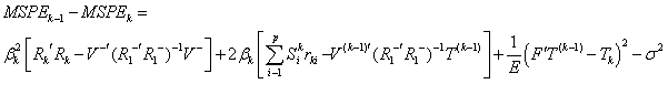 Dividing this
difference by E, and using the next equality
Dividing this
difference by E, and using the next equality 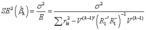 , we get that the kth
coefficient should remain in the model if:
, we get that the kth
coefficient should remain in the model if:
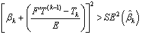 .
.
In the particular case where
all correlations are equal we get:
 , where
 ![]() and
and ![]() .
.
References
- Abramovich,
F. and Benjamini, Y.(1995), ‘ Thresholding of wavelet coefficients as
multiple hypotheses testing procedure’, in A. Antoniadis, ed., Wavelets
and Statistics, Vol. 103, Springer Verlag Lecture Notes in Statistics,
pp. 5-14.
- Abramovich,
F., Benjamini, Y., Donoho, D. and Johnstone, I. (2000) ‘Adapting to
Unknown Sparsity by Controlling the False Discovery Rate’, Technical
Report No. 2000-19, May 2000.
- Akaike, H.
(1973), ‘ Information theory and an extension of the maximum likelihood
principle.’ In Second International Symposium on information theory.
(eds. B.N. Petrov and F.Czaki). Akademia Kiadό, Budapest, pp. 267-281.
- Benjamini, Y.
and Hochberg, Y. (1995), ‘Controlling the false discovery rate: a
practical and powerful approach to multiple testing’, Journal of the
Royal Statistical Society, Series B. 57, 289-300.
- Benjamini, Y.
and Yekutieli, D. (1997) "The control of the False Discovery
Rate under dependence". Research Paper 97-4, Dept. of Statist. and
O.R., Tel Aviv University.
- Benjamini,
Y., Krieger, A. and Yekutieli, D. (2001), ‘Two Staged Linear Step Up
FDR Controlling Procedure’, Technical Report.
- Birgé, L. and
Massart, P. (2001), ‘ A Generalized Cp Criterion for Gaussian
Model," Technical Report, Lab. De Probabilitiés, Université
Paris VI.
- Cochran, W. G., (1977) Sampling Techniques, 3rd
edition, Wiley.
- Donoho ,D. L.
and Johnstone, I. M., (1994), ‘ Ideal Spatial Adaptation by Wavelet
Shrinkage’, Biometrika 81, no. 3, 425-455.
- Draper, N. R.
and Smith, H., (1998), Applied Regression analyses (Third Edition).
New York: Wiley.
- Foster, D.
and Stine, R., (1997), ‘ An Information Theoretic Comparison of Model
Selection Criteria’, Technical Report, Dept. of Statistics,
University of Pennsylvania.
- George, E. I.
and Foster, D. P. (1997), ‘Calibration and Empirical Bayes Variable
Selection’, Technical Report, University of Texas,
Austin.
- Mallows, C.L.
(1973), ‘ Some Comments on Cp’, Technometrics 12, 661-675.
- Salomon, O., Seligsohn, U., Steinberg, D.M.,Zalel, Y., Lerner, A., Rosenberg, N., Pshithizki, M., Oren, M., Ravid, B., Davidson, J., Schiff, E. and Achiron, R., (2004) The common prothrombotic factors in nulliparous women do not compromise blood flow in the feto-maternal circulation and are not associated with preeclampsia or intrauterine growth restriction, American Journal of Obstetrics and Gynecology , 2002-2009.
- Sarkar, S. (2002) Some Results on False Discovery Rate in Stepwise multiple testing procedures, Ann. Statist. 30, no. 1 , 239–257
- Tibshirani,
R. and Knight, K, (1999), ‘The Covariance Inflation Criterion For Adaptive
Model Selection’, J. R. Statist. Soc. B 61,Part 3, pp. 529-546.